Authors: Jackson Gold (jacksongold at berkeley.edu) and Nicolas Rault-Wang (nraultwang at berkeley.edu)

Credit to Notion for this template.

Neural Radiance Fields (NeRF)

Part 1: Fit a Neural Field to a 2D Image

Model Architecture

We created a Neural Field model with the recommended Multilayer Perceptron (MLP) network architecture. This model is trained to predict the RGB color for each pixel of an input image.

We normalize colors to $[0, 1]$ and encode each 2D pixel coordinate $x = (u,v)$ with a Sinusoidal Positional Encoding (PE) to help the model more easily distinguish neighboring pixels from each other. The PE of $x$ is given by

Training: fox.jpg

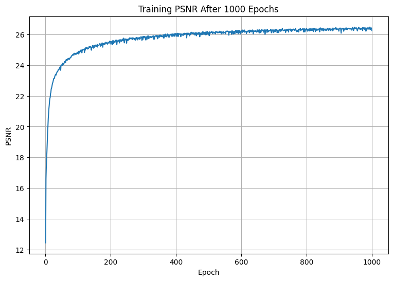
We trained the model to minimize the mean-squared error (MSE) in predicting the RGB colors for a randomly-selected batch of pixels from the input image. Thus, the model also maximizes the $PSNR = -10\times \log_{10}\left(MSE\right)$ of its reconstruction.

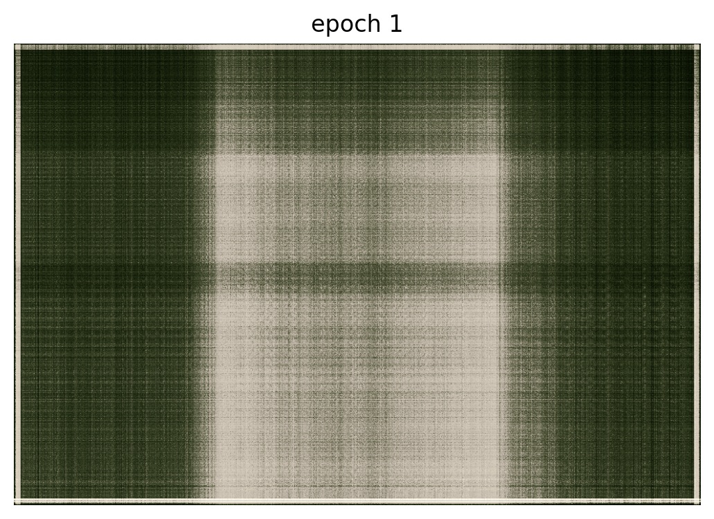
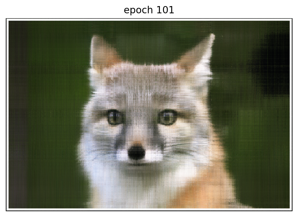
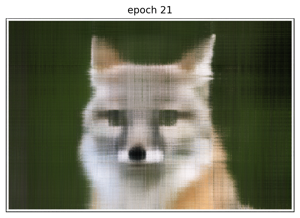
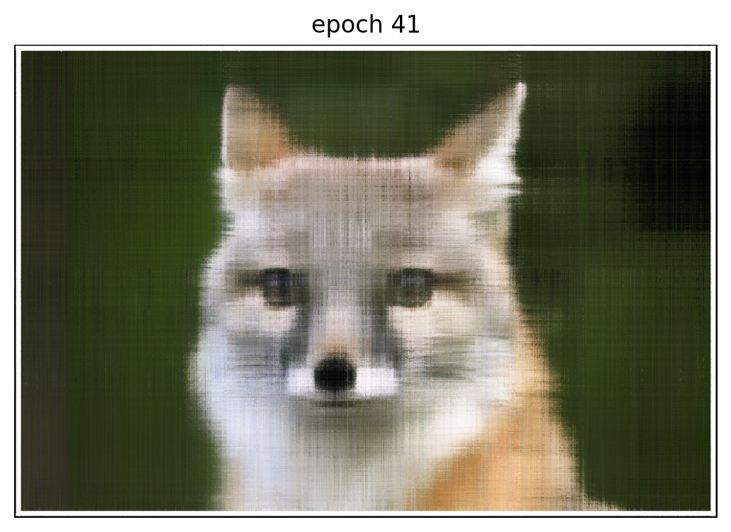
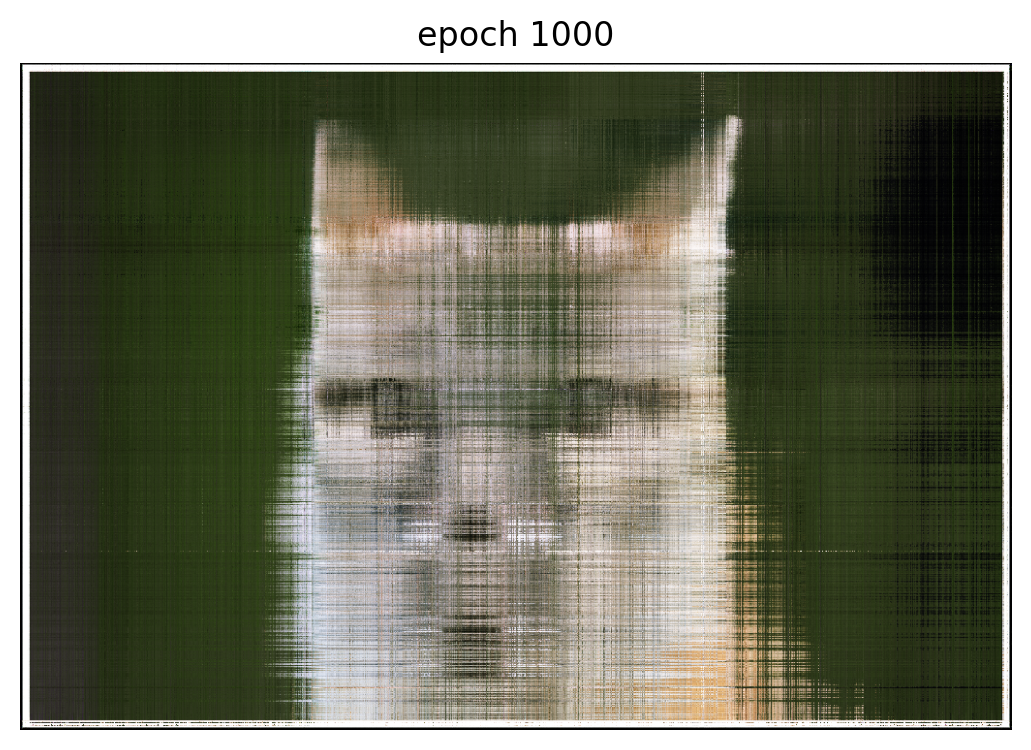
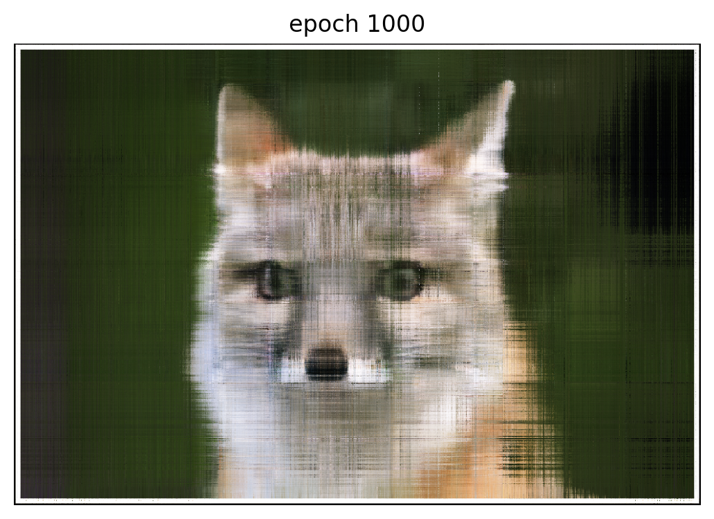
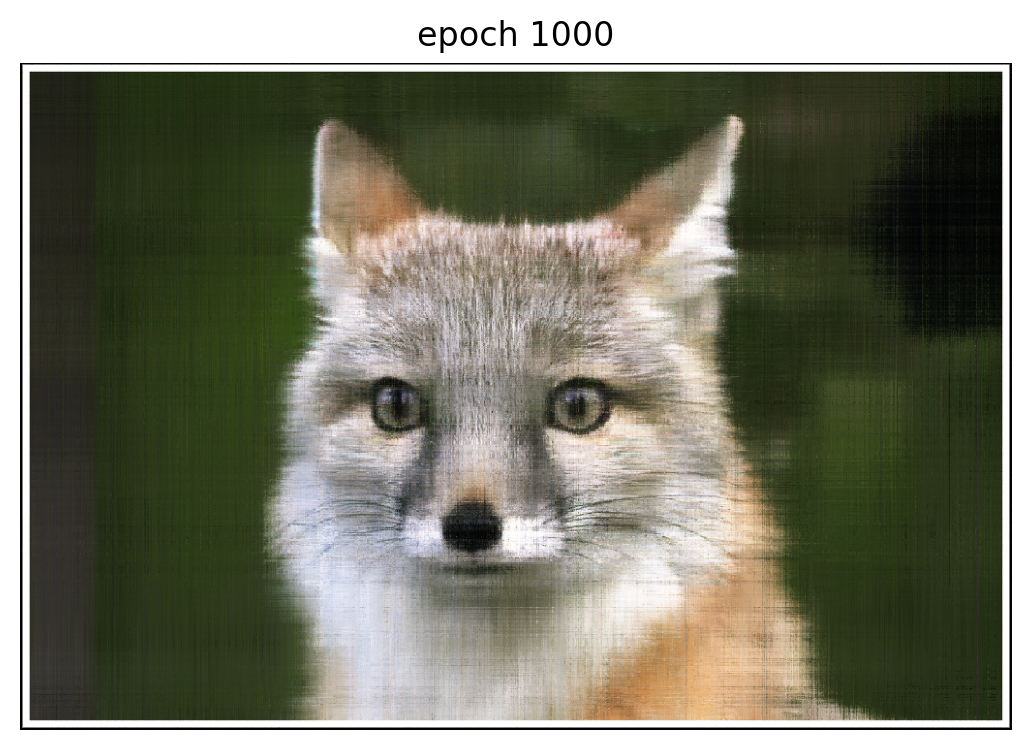
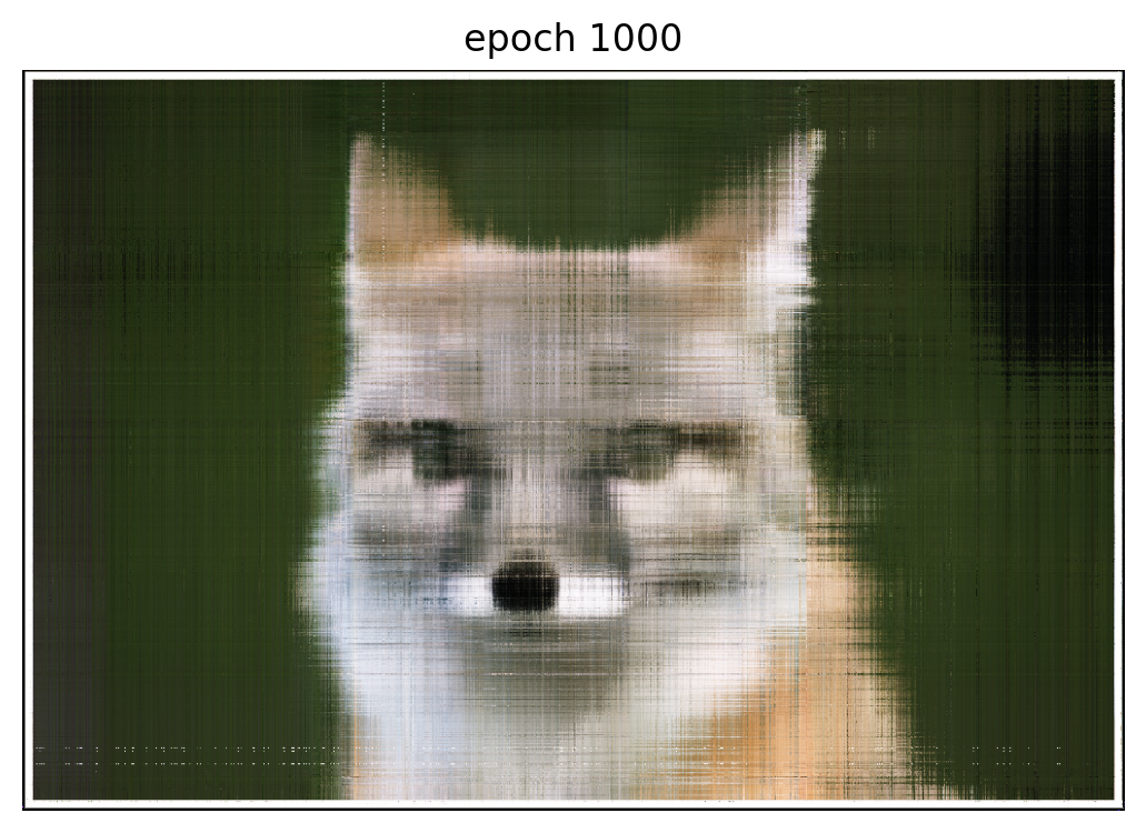
The figures below visualize over 1000 epochs with the Adam optimizer, learning rate $10^{-2}$, and batch size $10^4$.

Training hyperparameters

highest_frequency_level = 55
hidden dimension = 256
batch_size = 1e4
num_epochs = 1e3
learning_rate = 1e-2

Hyperparameter Tuning

We experimented different combinations of the max frequency $L$ for the positional encoding and the hidden dimension $D$ of each layer. All other hyperparameters were fixed to the values presented above.

We found that larger values of $L$ resulted in higher quality reconstructions for a smaller number of training iterations compared to smaller values of $L$. These smaller $L$ could achieve similar quality, but only after training for many more epochs. This suggests that a deeper positional components can help a neural field learn faster.

Fixing $L = 55$ we experimented with decreasing the number of hidden layers in the model from 256. We thought that the deep positional encoding made the learning problem substantially easier and would thus allow smaller models to perform well.

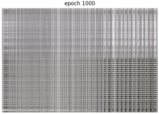
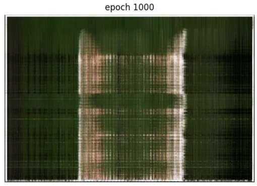
The figures above show that the model with $D = 128$ rendered only slightly lower quality versions of fox.jpg than $D= 256$. As we lowered $D$ to $64$ and $32$ the quality gets noticeably worse.

Interestingly, the renders for $L=55$ and $D = 32$ and $L=30$ and $D = 256$ are of similar quality, which may suggest that features provided by a high-dimensional positional encoding can be learned from a low-dimensional positional encoding by a more complex model.

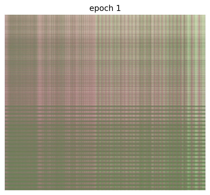
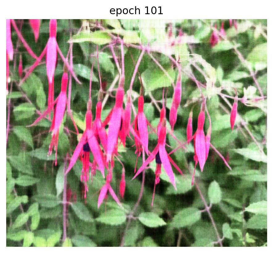
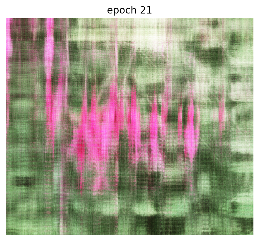
Training: fuchsia.png

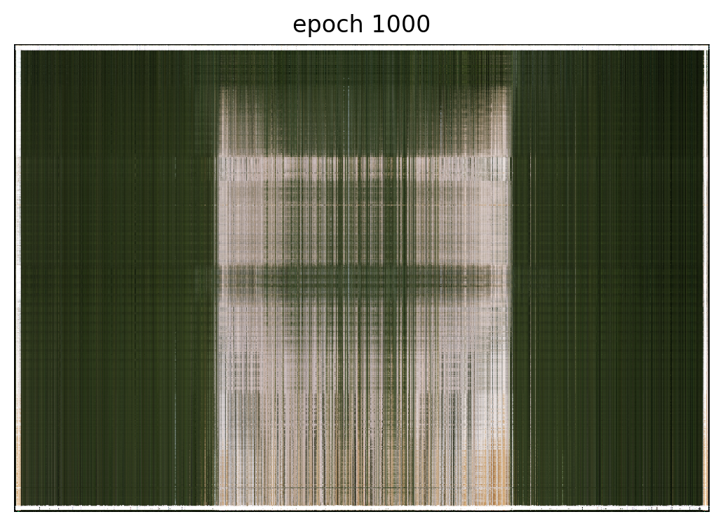
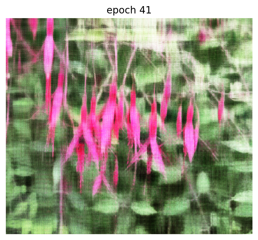
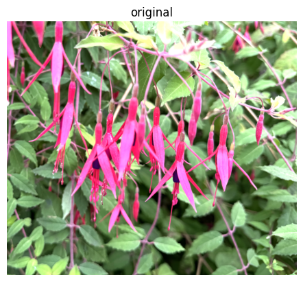
We needed to train a more complex model and use a deeper positional encoding for fuchsia.png to achieve good reconstructions. Our theory for why is that this image has more intricate details than fox.jpg.

Training hyperparameters

highest_frequency_level = 60
hidden dimension = 512
batch_size = 5e4
num_epochs = 500
learning_rate = 1e-3

Part 2: Fit a Neural Radiance Field from Multi-View Images

A Neural Radiance Field (NeRF) model learns the plenoptic function $F: \{x, y, z, \theta, \phi\} \rightarrow \{r, g, b, \sigma\}$ from a set of multi-view images captured by a set of calibrated cameras of a particular scene, enabling it to synthesize novel viewpoints. The original NeRF paper explains the concept in much greater detail.

Neural Radiance Field (NeRF) Model Architecture

This architecture is a deeper version of the model we used to represent 2D images in Part 1 because the 3D version of the learning task is more difficult. Specifically, given a camera view represented by a ray with origin $\vec r_o$ and direction $\hat r_d$, the model predicts the RGB color vector $\vec c_i = [r~~g~~b]$ and matter density $\sigma_i$ at each of $S$ discrete samples along that ray.

Each ray position $\vec r_o$ and direction $\hat r_d$ is augmented with sinusoidal positional encodings to help the model learn fine spatial details in a scene. Injecting $x$ and $r_d$ into later layers enables the model to “remember” input signals.

Creating Rays from Cameras

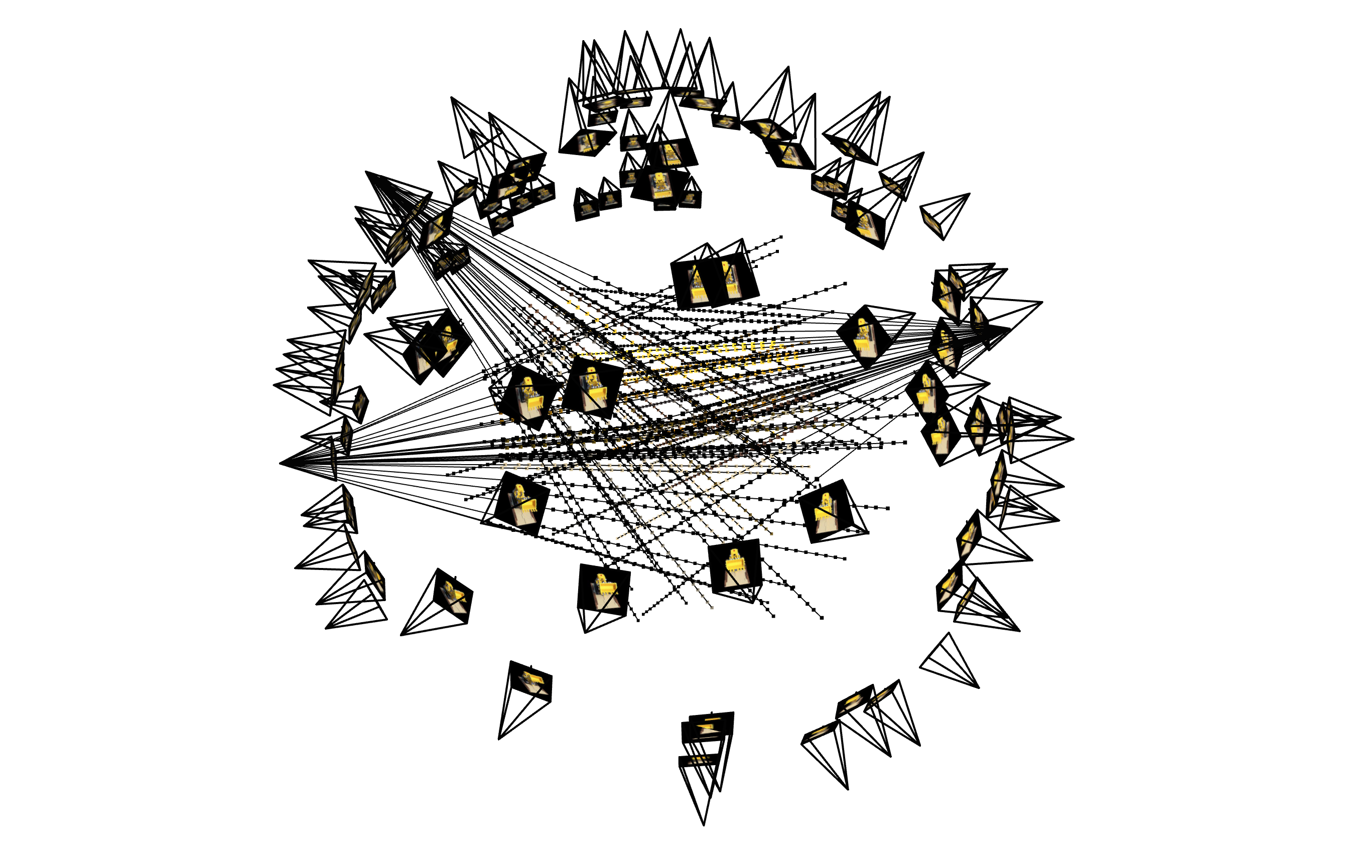
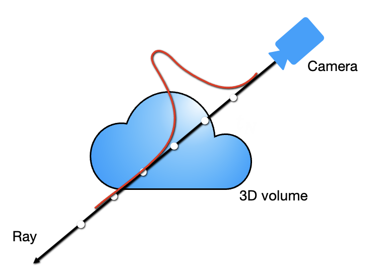
Each ray is characterized by an origin vector $\vec r_o$ in 3D world-coordinates and a normalized direction vector $\hat r_d$. Given a pixel $(u, v)$ viewed by a particular camera centered at $\vec r_o$, we can compute the ray that starts at $\vec r_o$ and passes through the center of $(u, v)$ in two steps:

1. Transform the pixel coordinate ($u, v)$ into camera coordinates $(x_c, y_c, z_c)$ by inverting the camera’s intrinsic matrix $K$, assuming focal length $(f_x, f_y)$ and principal point $(o_x, o_y) = (\frac{1}{2}\text{img width}, \frac{1}{2}\text{img height})$:

   $$\mathbf{K} = \begin{bmatrix} f_x & 0 & o_x \\ 0 & f_y & o_y \\ 0 & 0 & 1 \end{bmatrix}, \text{ where } \lambda \begin{bmatrix} u \\ v \\ 1 \end{bmatrix} = \mathbf{K} \begin{bmatrix} x_c \\ y_c \\ z_c \end{bmatrix} \\ \implies \begin{bmatrix} x_c \\ y_c \\ z_c \end{bmatrix} = \mathbf{K} ^{-1}\left(\lambda \begin{bmatrix} u \\ v \\ 1 \end{bmatrix}\right)$$

2. Transform the camera coordinate $(x_c, y_c, z_c)$ into world coordinates $(x_w, y_w, z_w)$ by inverting the camera’s extrinsic matrix, defined by a rotation matrix $\mathbf R_{3\times 3}$ and a translation vector $\mathbf t$:

Ray Sampling

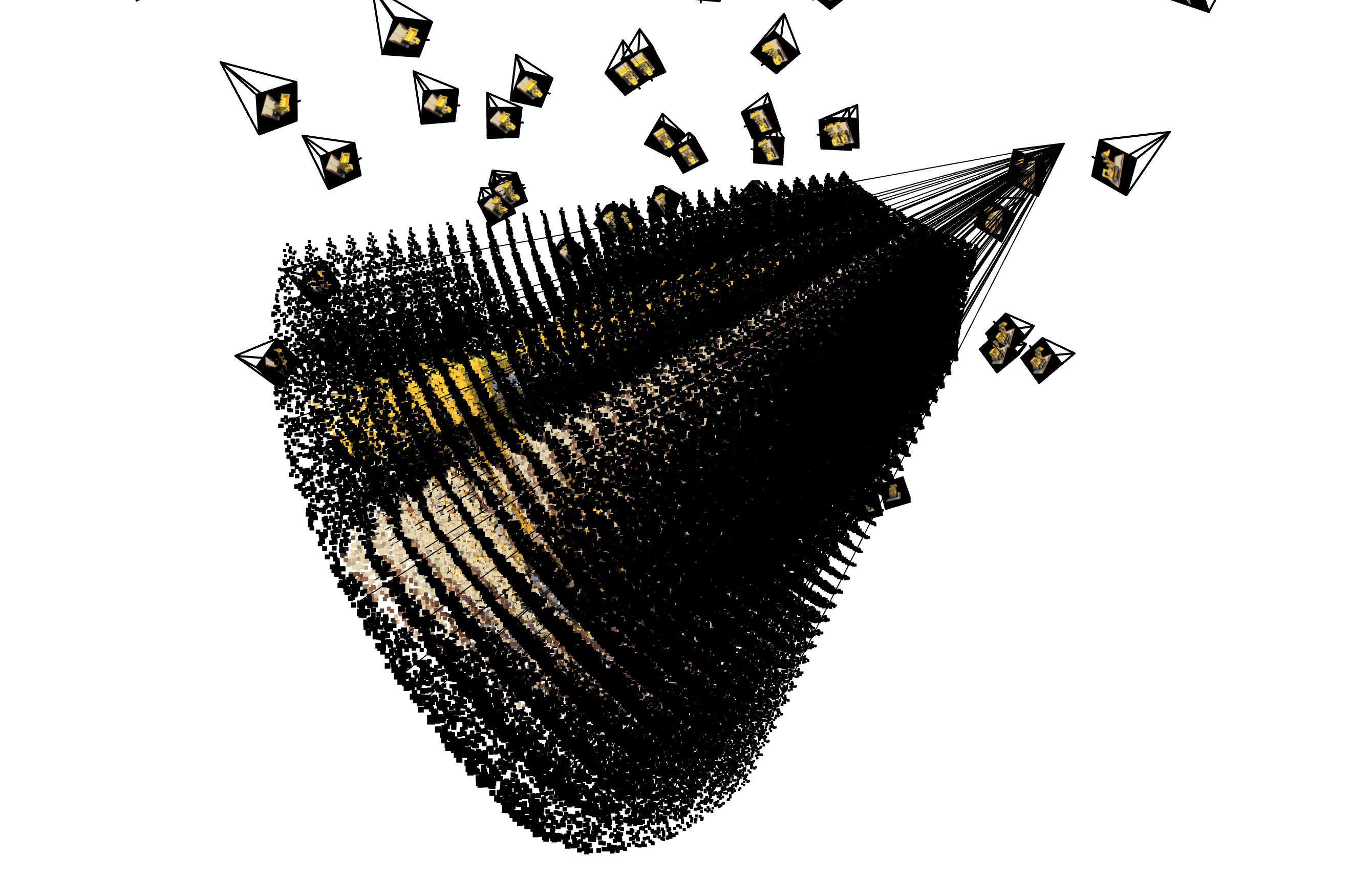
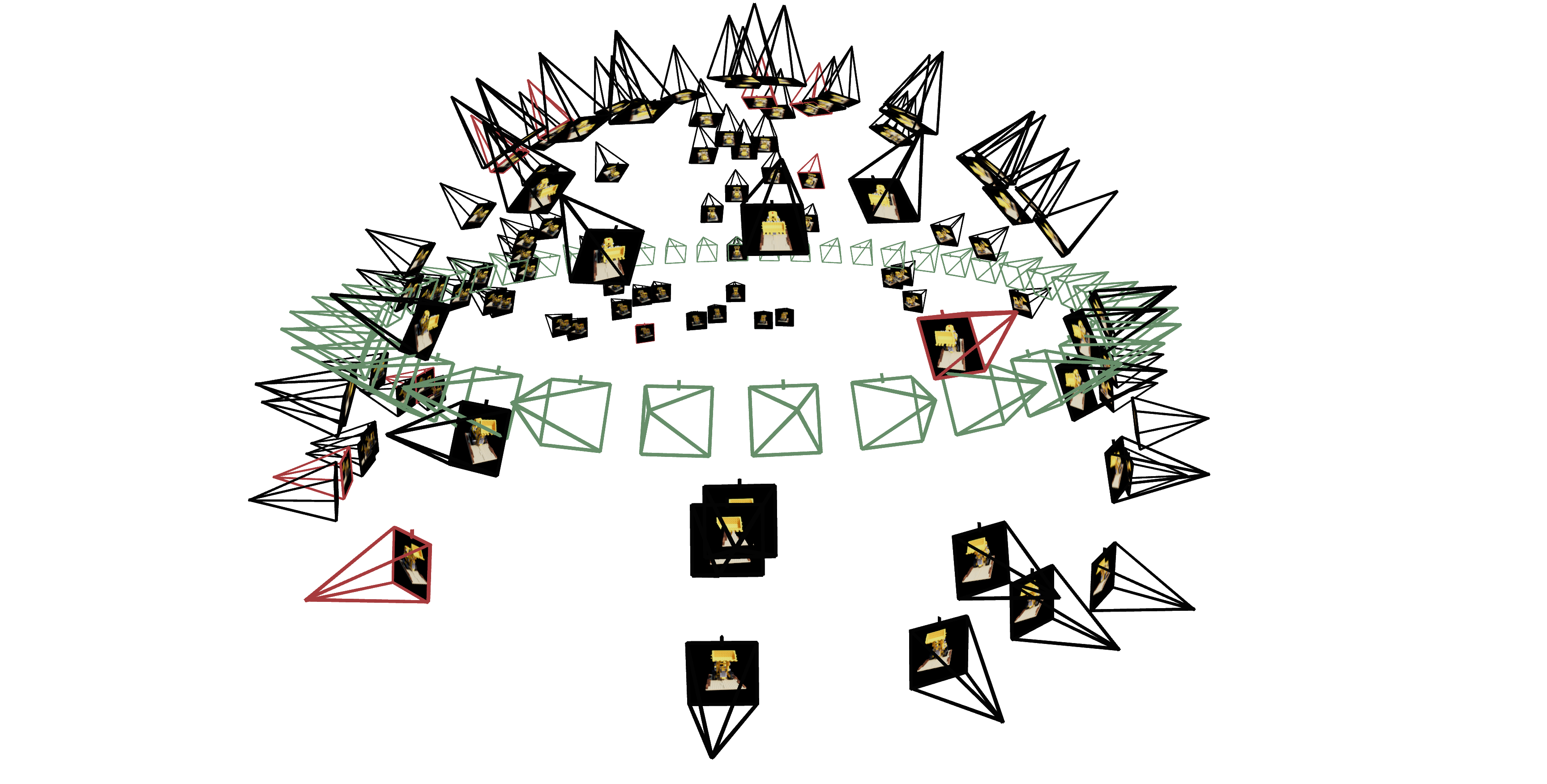
Our training set consists of $N$ rays evenly sampled from the calibrated training cameras. For computation, we represent each ray as a vector of $S$ discrete points along the portion of the ray that passes through the volume of the scene.

Volumetric Rendering

We estimate the color $\hat{{C}}(\vec r_o, \hat r_d)$ observed by a ray view $(\vec r_o, \hat r_d)$ with a discrete approximation to the volume rendering equation, which weighs the predicted color contribution $\vec c_i$ from the $i$th sample point by transmittance probabilities based on the predicted densities $\{\sigma_j\}_{j=1}^{i-1}$ between $i$ and $\vec r_o$.

Here, $T_i$ is the transmittance probability that the ray does not terminate before the $i$th sample, $\alpha_i$ is the probability that the ray terminates at the $i$th sample, and $\delta_i$ is the distance between samples $i$ and $(i-1)$.

While we set $\delta_i$ to a constant step size when rendering a novel view, more sophisticated methods like coarse-to-fine sampling adjust $\delta_i$ to focus sampling points around the solid objects of the scene.

Training Hyperparameters

Dataset Parameters:
    number of sampled rays = 100 * 45_000
    number of cameras = 30
    number of samples per ray = 32
    sample point perturbation = 0.02

Model Parameters
    number of hidden layers = 256
		highest positional encoding frequency for ray sample position = 10
		highest positional encoding frequency for ray sample direction = 4
    batch size (number of rays) = 10_000
    training epochs = 1000
    Adam Optimizer learning rate = 5e-4

Training Visualization

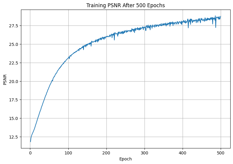
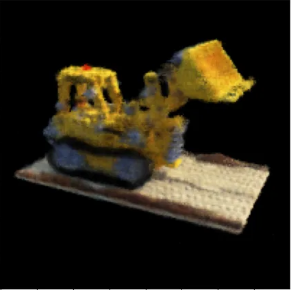
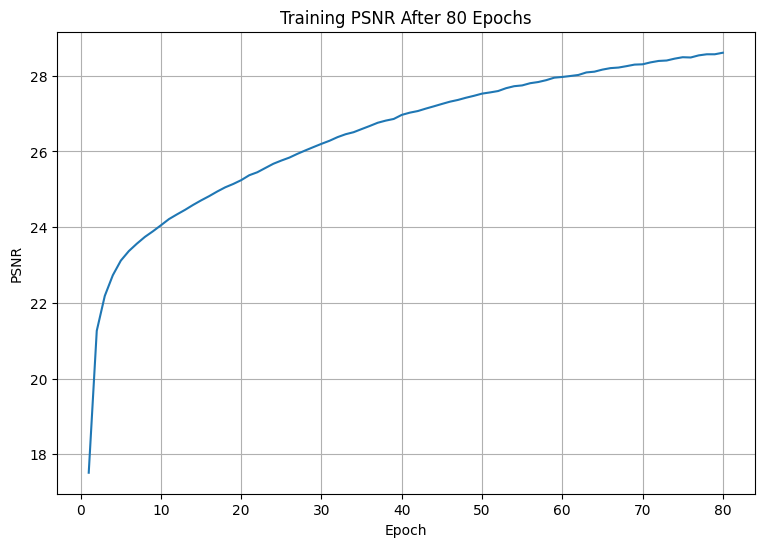
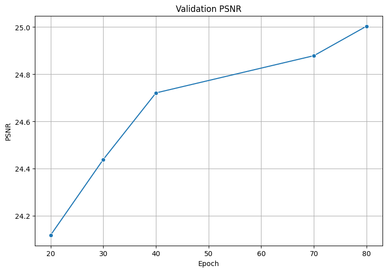
We applied our model to synthesize the same training view every 10 epochs during training to visualize the optimization process. Plots of training and validation PSNR are shown below.

Rendering Novel Views

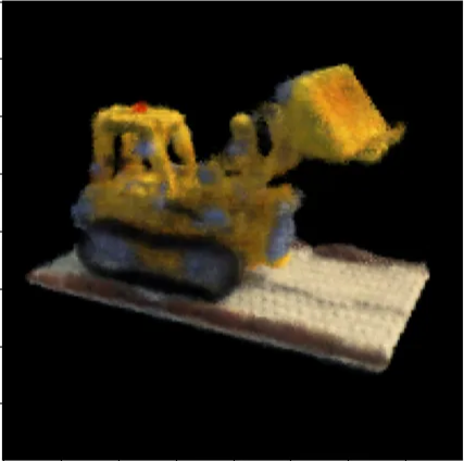
To render a novel camera’s view, we estimate the color of every pixel in that camera’s image using our NeRF model and the volumetric rendering equation. After rendering views from the test set of spherically-arranged cameras (see the right figure in Ray Sampling), we can make a video that shows the model spinning around:

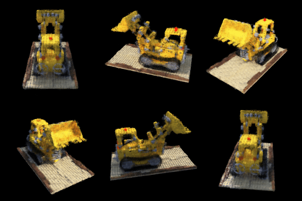
In more detail, to render a given pixel $(u, v)$, we begin by computing the ray $(\vec r_o, \hat r_d)$ that starts at the camera center and passes through the center of pixel (see Creating Rays from Cameras). Applying the model to $S$ sample points along this ray yields estimates of the colors $\{\vec c_i\}_{i=1}^S$ and densities $\{\sigma_i\}_{i=1}^S$ at these points, which we plug into the volumetric rendering equation to obtain an estimate $\hat C(\vec r_o, \hat r_d)$ of the color of $(u, v)$. Repeating this calculation for each of the 40k pixels yields a $200\times200$ image render of the novel view.

Part 3. Bells & Whistles

Depth Maps

To render a depth map of the scene, we compute the expected depths $\hat t$ visible by each pixel in a view, normalized to $[0, 1]$, then color pixels with large $\hat t$ reddish, medium $\hat t$ blackish, and small $\hat t$ bluish. After render a depth map for each test camera (see the last figure in Ray Sampling), we can form a video showing a depth-map of the model from different angles.

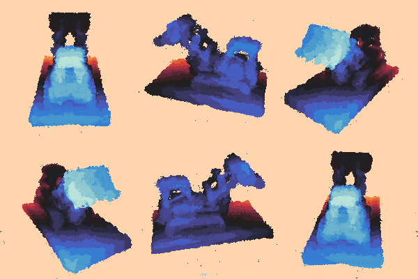
We estimate the expected depth $\hat t$ between $\vec r_o$ and a scene point with a volumetric rendering equation similar to the one we used for color, but with a scalar depth $t_i$ in place of a color $\vec c_i$.

Facial Keypoint Detection with Neural Networks

Part 1: Nose Tip Detection

We created a pipeline to detect nose tips in facial images using the IMM Face Database. Images were preprocessed into grayscale, normalized, and resized, with a custom PyTorch dataloader handling data loading and annotations. A CNN with 4 convolutional layers, max pooling, and ReLU activation extracted features, followed by fully connected layers predicting normalized nose tip coordinates, and finally a sigmoid activation function. The model was trained using mean squared error loss and the Adam optimizer, with hyperparameter tuning to optimize performance.

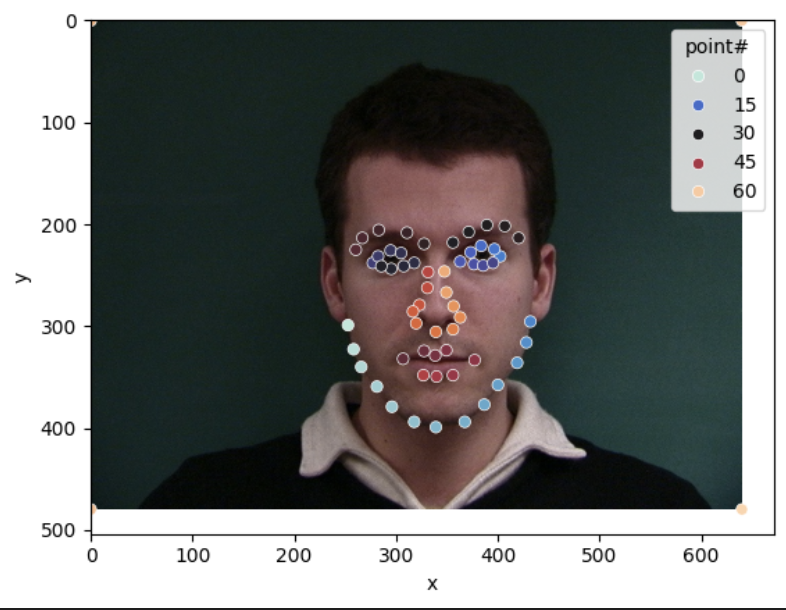
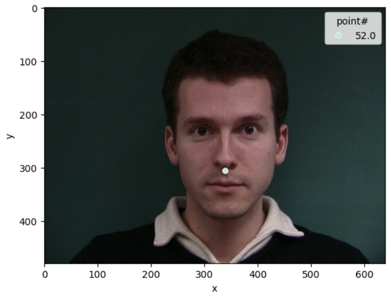
Visualizing Ground-Truth Keypoints

A sampled image from the dataloader was visualized along with its ground-truth keypoints to ensure the data pipeline and annotations were correctly implemented. The visualization confirms that the keypoints align accurately with their respective facial features, indicating the integrity of the dataset.

Training and Validation Loss

The Mean Squared Error (MSE) loss was tracked for both the training and validation datasets throughout the training process. A plot of the training and validation losses shows a consistent downward trend, indicating that the model is learning effectively. However, the gap between training and validation losses was monitored to avoid overfitting.

Network Configuration and Experimentation

During the development process, various network configurations were explored. These included testing different architectures with 3-4 convolutional layers, adjusting the number of channels in convolutional layers, incorporating a learning rate scheduler to dynamically adjust the learning rate, and experimenting with different learning rates, such as 5e-4.

Despite these adjustments, the model’s performance remained relatively unchanged. The breakthrough came when the output of the model was passed through a sigmoid activation layer. This normalized the predictions to the range of 0 to 1, aligning them with the ground-truth data distribution. After this modification, the model began performing effectively, demonstrating the importance of output normalization in this task.

Correct and Incorrect Predictions

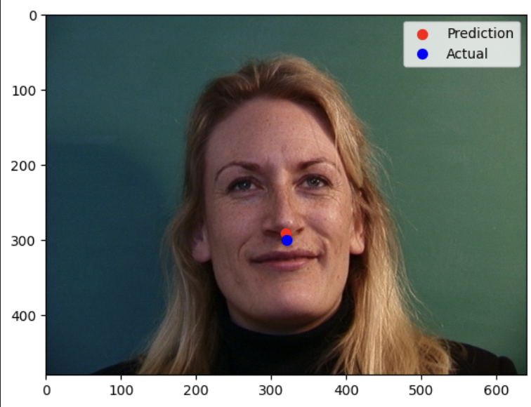
Correct Predictions

Two images were identified where the network correctly detected the nose tip keypoint. In these cases, the images had clear, well-lit facial features, and the nose tip was positioned centrally within the image, making it easier for the network to localize.

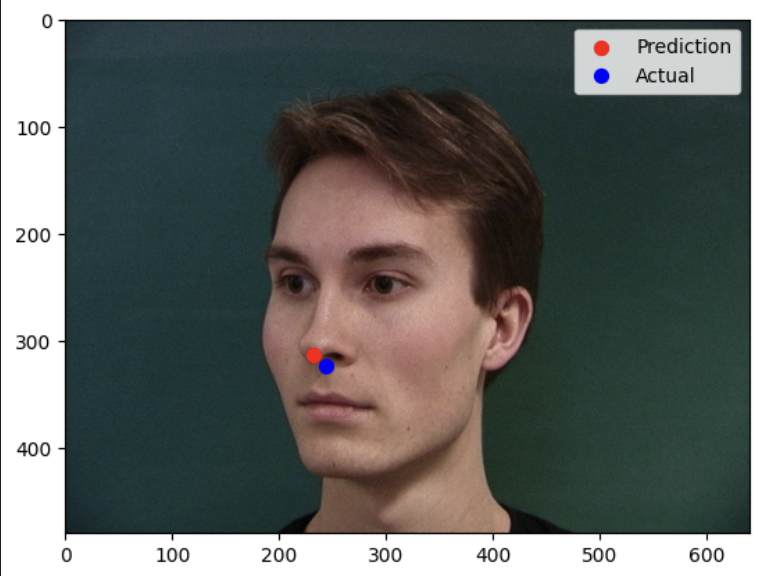
Incorrect Predictions

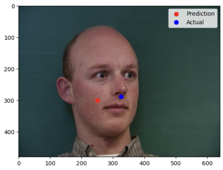
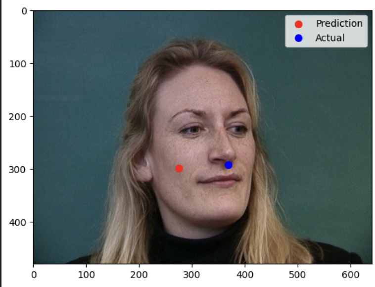
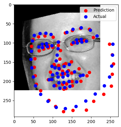
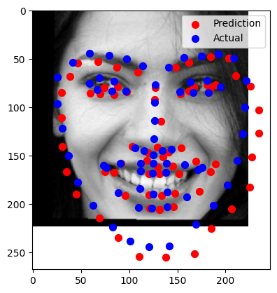
Two images were identified where the network failed to detect the nose tip keypoint accurately. Possible reasons for these failures include occlusion, where parts of the face, including the nose tip, and unusual angles or expressions, where the face in the image was captured at an angle or had an exaggerated expression, deviating significantly from the training data.

These observations highlight areas for potential improvement in the dataset and model robustness, such as augmenting the training data with more diverse angles, lighting conditions, and facial expressions to improve generalization.

Part 2: Full Facial Keypoints Detection

Sampled Image with Ground-Truth Keypoints

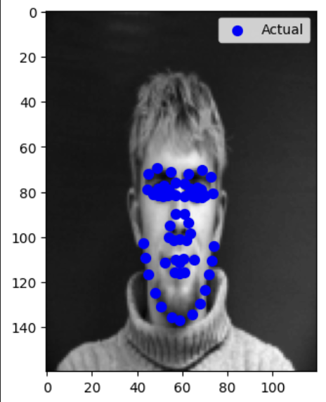
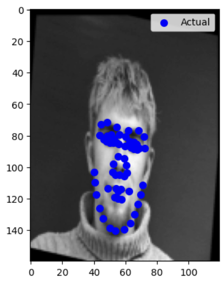
To ensure the data pipeline correctly handles all 58 keypoints, sampled images from the dataloader were visualized with their respective ground-truth keypoints. After incorporating data augmentation (random brightness adjustment, rotation, and shifting), the keypoints were adjusted dynamically to align with the transformations. Initial overfitting issues were resolved once augmentations were implemented correctly. This step validated the integrity of the dataset and transformations.

Model Architecture and Training Details

The network architecture was updated to accommodate larger input images and the increased output size for 58 keypoints (116 coordinates). Key details of the architecture include:

• Convolutional Layers: Six layers with increasing channel sizes (16 → 128), each followed by batch normalization and ReLU activation.

• Pooling: MaxPooling layers to downsample spatial dimensions progressively.

• Fully Connected Layers: A dense layer (256 units) followed by dropout (30%) and output normalization with a sigmoid activation for the final layer.

• Hyperparameters:
  • Optimizer: Adam with a learning rate of $1×10^{−3}$.
  • Scheduler: Exponential decay with a factor of 0.9.
  • Loss Function: Mean Squared Error (MSE).

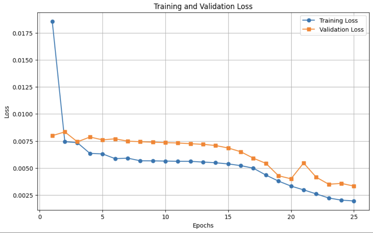
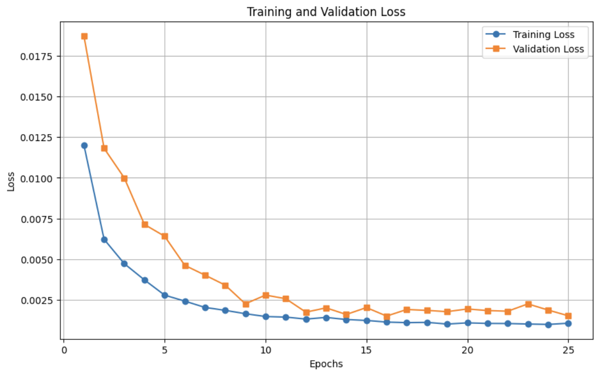
Training ran for 25 epochs with a batch size of 32 for both training and validation datasets. The learning curve shows a downward trend in both training and validation loss, confirming effective learning post-augmentation fixes.

Training and Validation Loss Plot

The plot below illustrates the loss trends across epochs, with a steady convergence and minimal gap between training and validation loss.

Correct and Incorrect Predictions

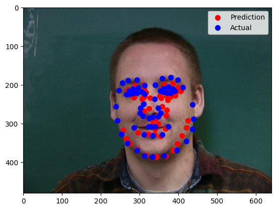
Correct Predictions

Two images were identified where the network correctly detected the nose tip keypoint. In these cases, the images had clear, well-lit facial features, and the nose tip was positioned centrally within the image, making it easier for the network to localize.

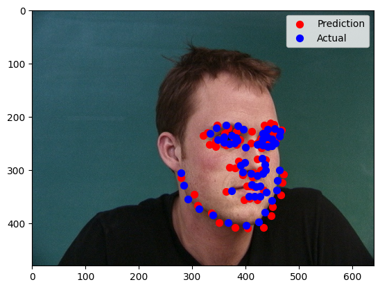
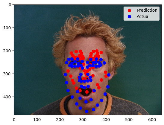
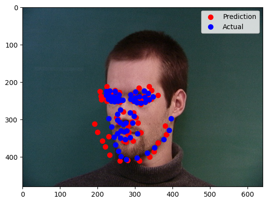
Incorrect Predictions

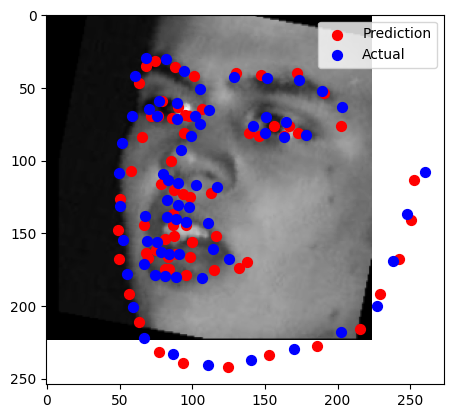
Two images were identified where the network failed to detect the keypoints accurately. Possible reasons for these failures include occlusion, where parts of the face, and unusual angles or expressions, where the face in the image was captured at an angle or had an exaggerated expression, deviating significantly from the training data.

These errors suggest the need for further data augmentation to cover occlusion and angle variations and potentially incorporating attention mechanisms for improved robustness.

Learned Filters

Filters learned in the initial convolutional layers captured basic edge and gradient patterns, which are critical for identifying facial structures. Deeper layers focused on more complex features, reflecting the hierarchical nature of the model. Visualization of these filters highlights their capacity to detect both general and specific facial attributes.

Part 3: Train with Larger Dataset

Architecture and Training Details

For this part, the architecture was updated to use ResNet18, a standard CNN model, with the following modifications:

• First Layer: Changed to accept single-channel grayscale images (input channels = 1).

• Last Layer: Output channel set to 136 to predict 68 keypoints, each with x,y coordinates.

  x,yx, y

Training Hyperparameters:

• Dataset: iBUG Face in the Wild dataset, resized cropped faces to 224×224.

• Batch Size: 64

• Optimizer: Adam with a learning rate of $1×10^{−3}$.

• Loss Function: Mean Squared Error (MSE)

• Epochs: 25

• Device: GPU (Colab environment)

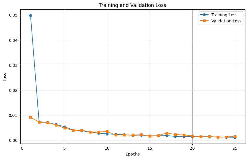
Training and validation losses were plotted to observe convergence. The learning curve showed consistent improvement, with validation loss tracking closely to the training loss, indicating minimal overfitting.

Training and Validation Loss Plot

Visualized Keypoints on Testing Set

The trained model was used to predict keypoints on the test dataset. Several images were sampled and visualized with their predicted keypoints overlaid. Predictions were converted from normalized values (relative to the resized 224×224 to absolute pixel coordinates in the original image to match the test dataset format.

Testing on My collection

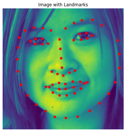
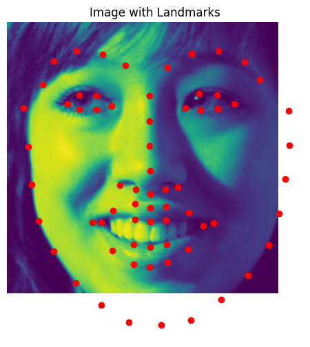
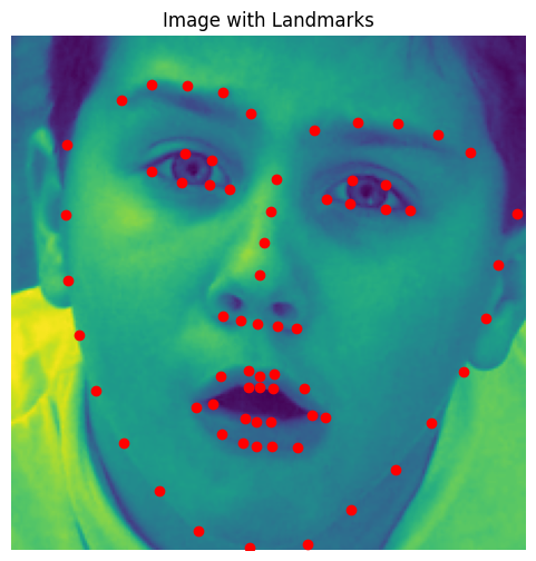
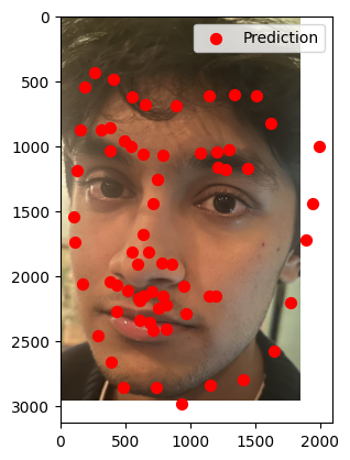
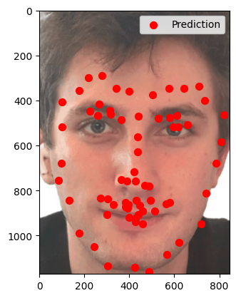
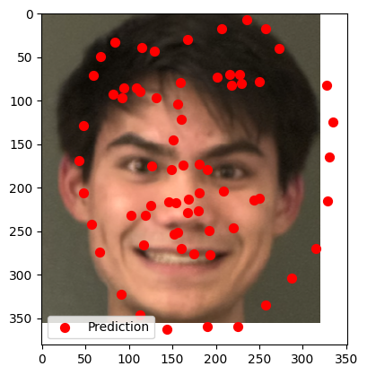
The model was tested on three photos from my collection to assess its performance on unseen, real-world data. Here’s a summary of the results:

1. Photo 1 (Success):
   • Clear, frontal images with standard facial features.
   • Keypoints aligned well with major landmarks, including eyes, nose, and mouth.

1. Photo 2 (Partial Success):
   • Side profile with slight occlusion from hair.
   • Keypoints predicted reasonably well but showed minor misalignment around the jawline.

1. Photo 3 (Failure):
   • Photo with exaggerated facial expression and low lighting.
   • Significant deviations in keypoint positions, particularly around the mouth and chin.

These observations highlight the strengths and limitations of the model:

• Strengths: Accurate predictions for well-lit, frontal images with minimal occlusion.

• Weaknesses: Struggles with extreme poses, poor lighting, and occlusions.

Part 4: Pixelwise Classification

Heatmap Distribution and Parameters

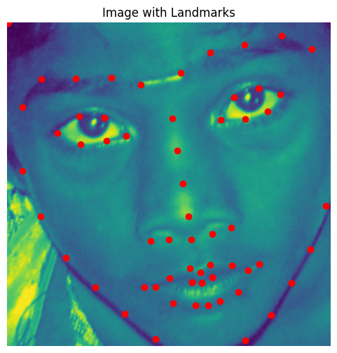
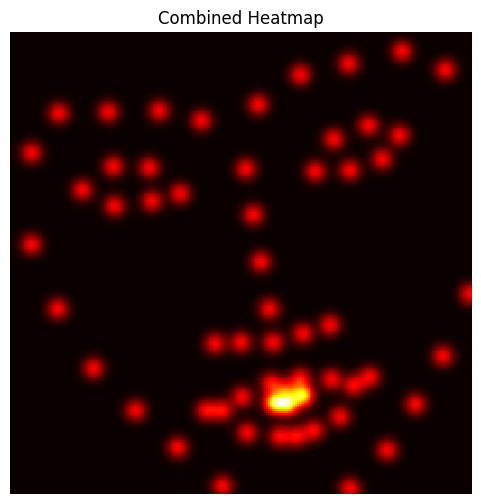
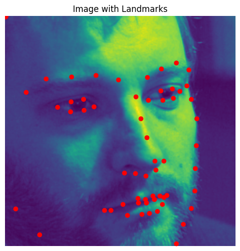
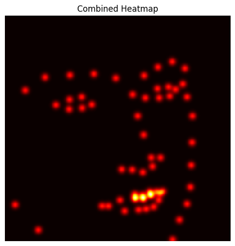
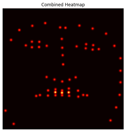
To convert keypoint coordinates into pixel-aligned heatmaps for training, 2D Gaussian distributions were used. Each ground-truth keypoint was represented by a Gaussian centered at its corresponding coordinate on the map. The key parameters for generating heatmaps were:

• Sigma: The standard deviation of the Gaussian, controlling the spread around the keypoint. A smaller sigma (e.g.,  $\sigma$ = 2 ) was chosen for sharp and localized keypoints.

• Resolution: Heatmaps were aligned with the resized input image dimensions (224x224).

The resulting heatmaps served as the ground truth for supervision. Weighted averages were later used to extract the predicted coordinates from the generated heatmaps.

Accumulated Heatmaps for All Landmarks

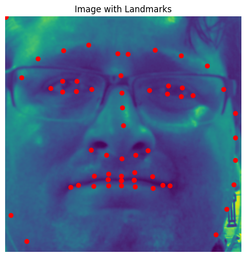
For three images, the accumulated heatmaps for all 68 keypoints were visualized to observe the network’s understanding of landmark distribution. These visualizations confirmed the heatmaps accurately captured key facial features.

Model Architecture and Training Details

For this task, the U-Net architecture was employed, pre-trained on segmentation tasks and fine-tuned for facial keypoint detection. Key modifications included:

• Input Layer: Adapted to accept single-channel grayscale images (1 input channel).

• Output Layer: Adjusted to predict 68 heatmaps, one for each keypoint.

Architecture Details:

• Encoder: Pretrained convolutional layers to extract hierarchical features.

• Decoder: Transpose convolutional layers for pixel-aligned output.

• Output Channels: Set to 68, representing individual heatmaps for each keypoint.

Training Hyperparameters:

• Loss Function: MSE between predicted and ground-truth heatmaps.

• Learning Rate: $1 \times 10^{-3}$

• Batch Size: 64

• Epochs: 5

• Optimizer: Adam

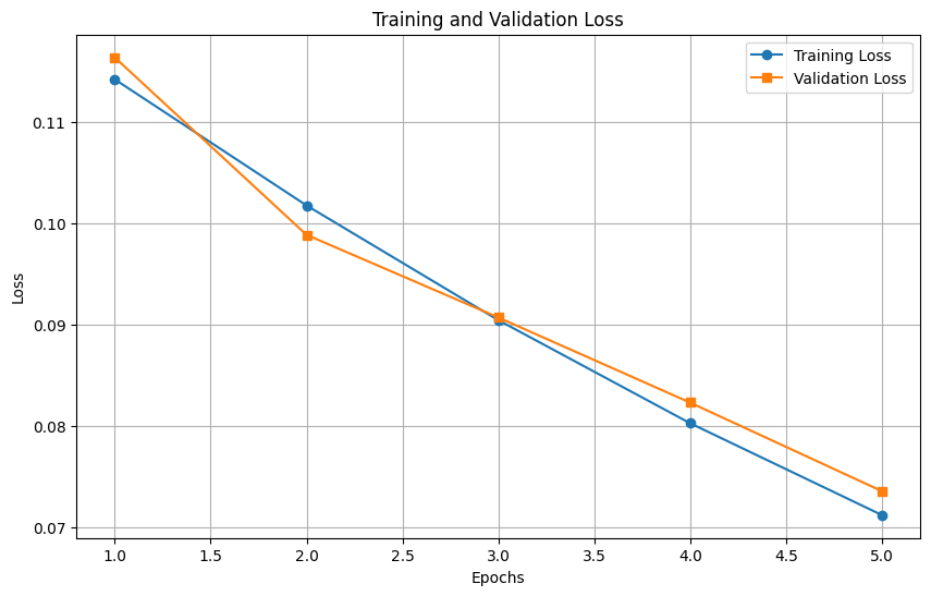
Training and validation loss were plotted over 5 epochs, showing convergence and minimal overfitting.

Training and Validation Loss Plot

Keypoint Predictions on Test Set

Two images from the test set were visualized with predicted keypoints. Heatmap predictions were converted back to keypoint coordinates using weighted averages of heatmap activations. The keypoints aligned closely with the facial features, demonstrating the model’s pixelwise classification effectiveness.

Testing on Personal Photos

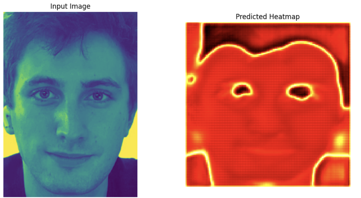
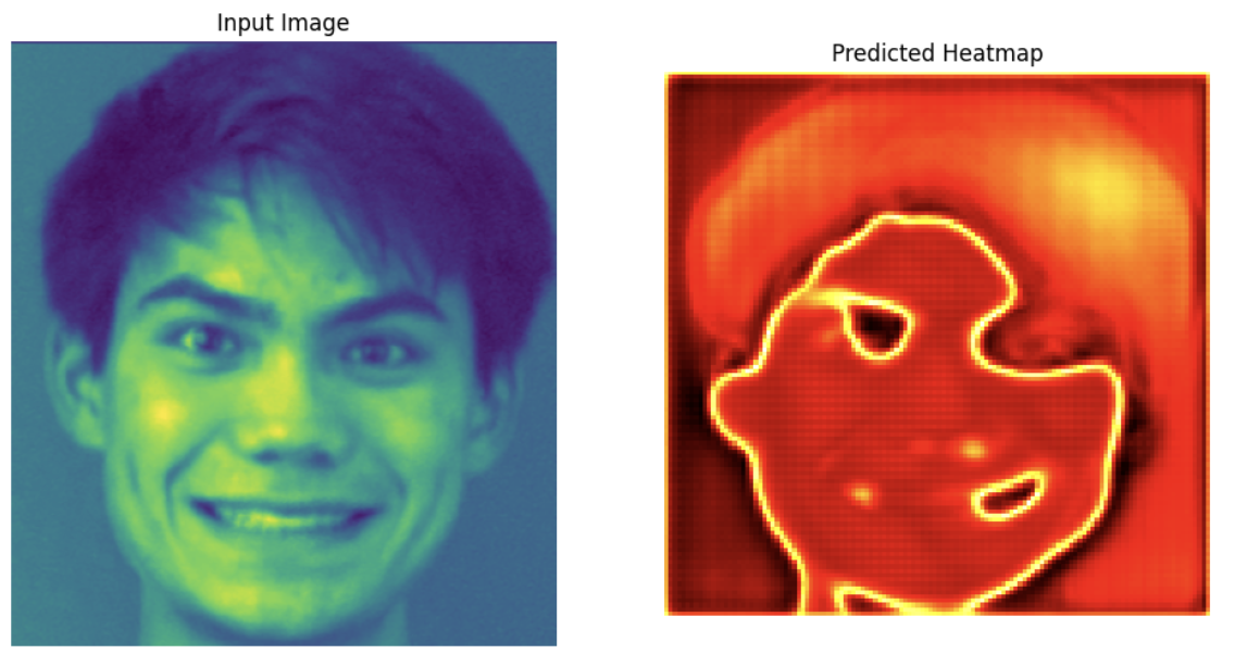
The trained model was evaluated on three photos from my collection:

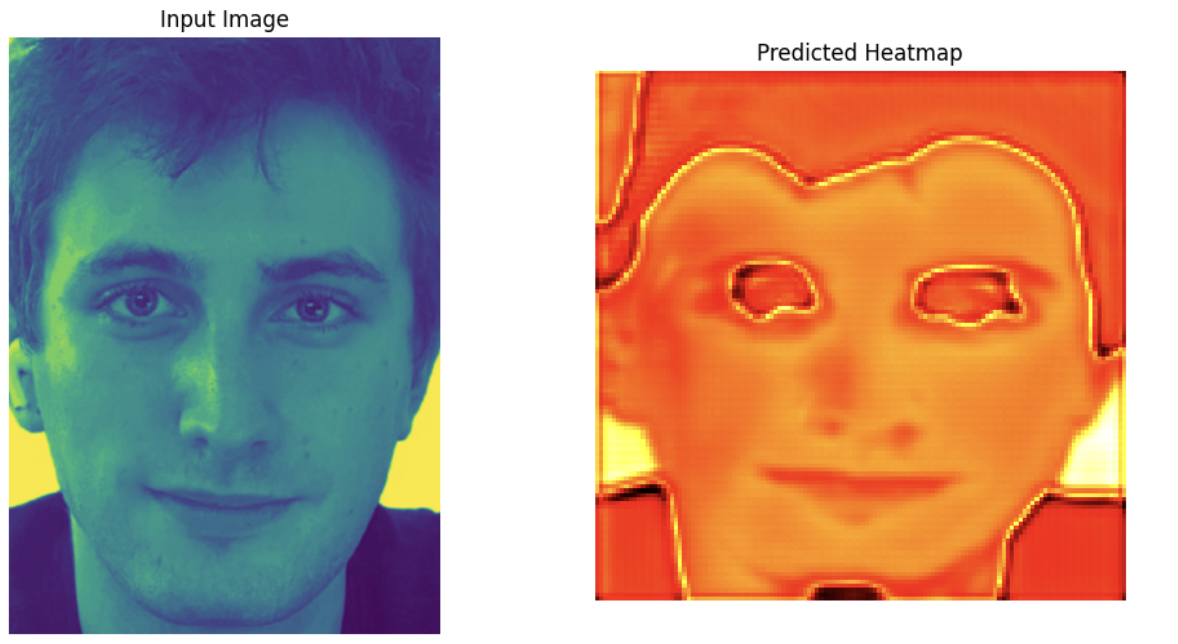
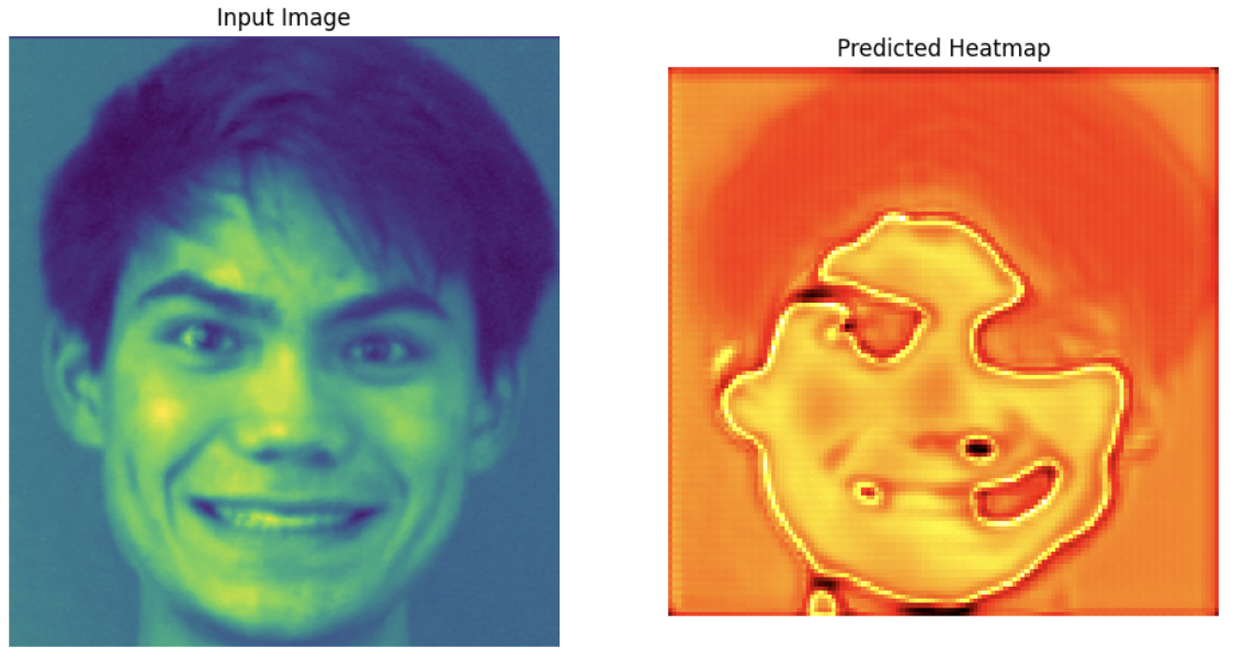
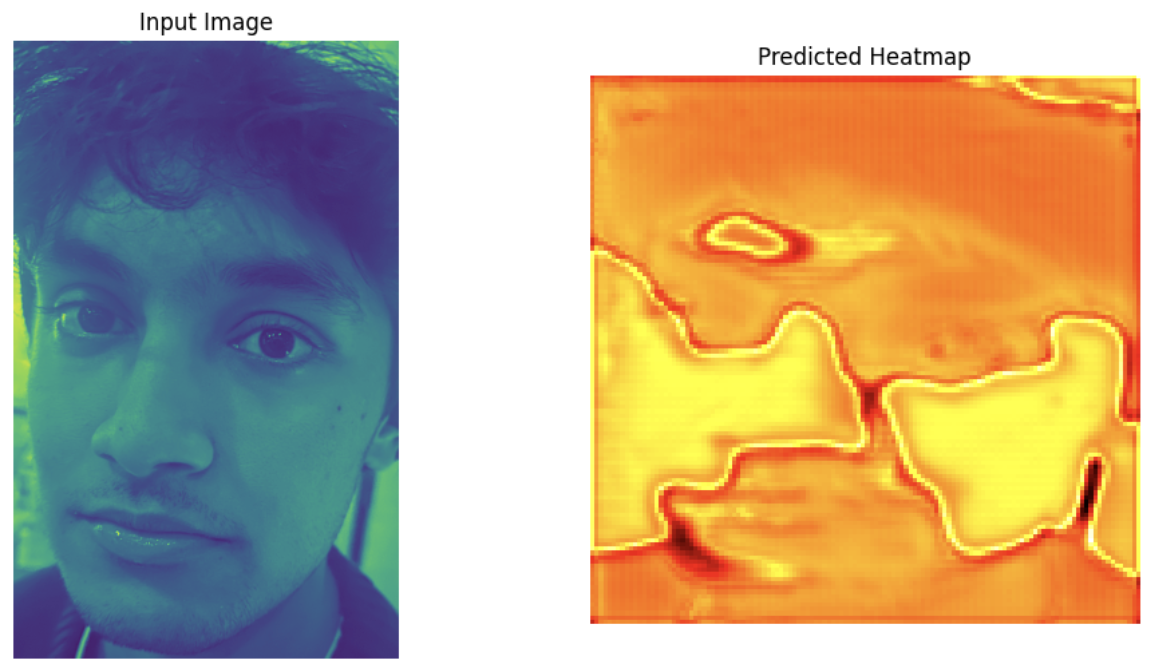
Bells and Whistles: 1 and 0 Mask Heatmaps

The Gaussian heatmaps were replaced with binary mask heatmaps, where each keypoint location was assigned a value of 1, and all other pixels were assigned 0. This modification simplifies the ground truth but eliminates the smooth gradient provided by Gaussian distributions, which may affect the network’s ability to generalize.

Training Process

• Mask Generation: Binary masks were created for each keypoint, with a single pixel at the keypoint’s location set to 1, and all other pixels set to 0.

• Loss Function: MSE loss was retained for consistency.

• Other Parameters: The training process (architecture, optimizer, learning rate, etc.) remained unchanged from the original setup with Gaussian heatmaps.

Training and Validation Loss Plot

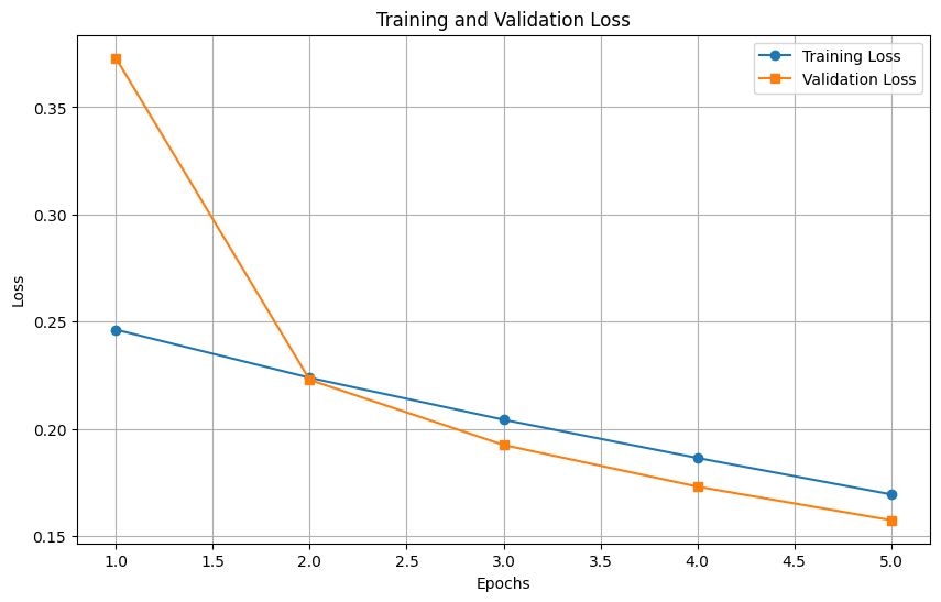
Observations:

• The loss curve converged more slowly compared to Gaussian heatmaps.

• Validation loss stagnated after initial improvement, suggesting limited learning capacity.

Some Examples:

Why It Probably Did Not Work as Well

1. Lack of Gradient Information:

Binary masks provide no gradient or spatial distribution for the keypoints, unlike Gaussian heatmaps, which offer a smooth, localized representation. This limits the network’s ability to learn the precise location of keypoints.

2. Pixel-Level Sensitivity:

A single-pixel target is highly sensitive to shifts, making it challenging for the network to predict exact locations, especially for smaller or occluded features.

3. Poor Generalization:

The absence of spatial information in binary masks reduced the model’s ability to generalize to unseen poses, angles, and expressions.