
CS180 Project 2: Fun with Filters and Frequencies!
Author: Nicolas Rault-Wang (nraultwang at berkeley.edu)
Credit to Notion for this template.
Part 1: Fun with Filters
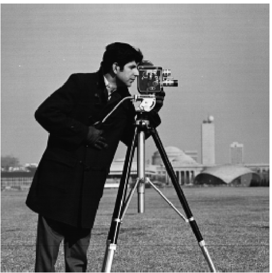
- In this part, we’ll take x and y partial derivatives of the “cameraman” image, , by convolving it with the finite difference filters and .
- To see the effects of first applying a gaussian filter , we’ll take these partial derivatives of without (part 1.1) and before (part 1.2) smoothing.
- We’ll use the following notation:
Part 1.1: Finite Difference Operator
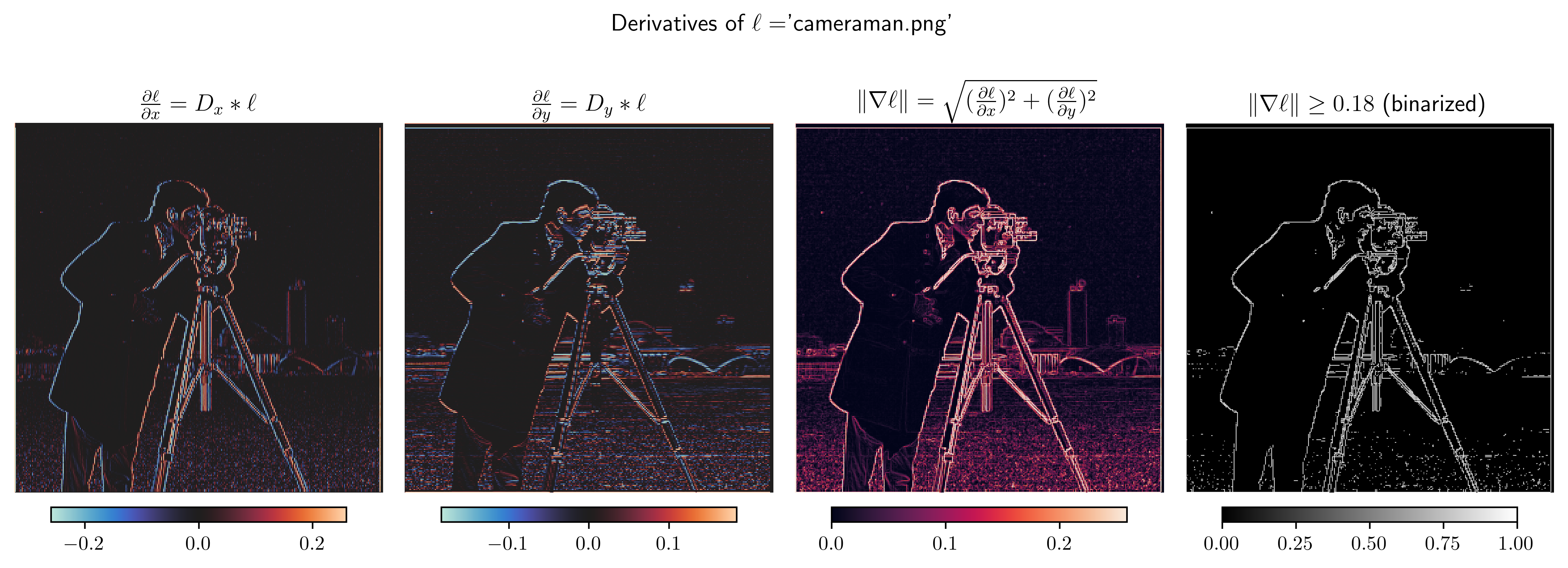
- The gradient magnitude image, , is formed by computing the magnitude of the gradient at every position in the image.
where and are computed by convolving with the finite difference filters and , respectively.
- To create an edge detection image, we select a threshold and at each position evaluate whether . The result is an image of the same shape as where a pixel value of 0 corresponds to the absence of an edge in and a pixel value of 1 corresponds to the presence of an edge in .
Part 1.2: Derivative of Gaussian (DoG) Filter
- We smooth with before taking its x and y partial derivatives. We’ll demonstrate that this operation is equivalent to a single convolution with and , respectively.

- Comparing the non-smoothed derivatives to the gaussian-smoothed derivatives of , we see that smoothed derivatives and edge detections are less noisy, and appear to have a higher SNR. However, one cost smoothing is less-localized edge detections because edges that look like step functions in the original image and the un-smoothed derivatives are more gradual and occur over a large spatial extent in the smoothed derivatives.
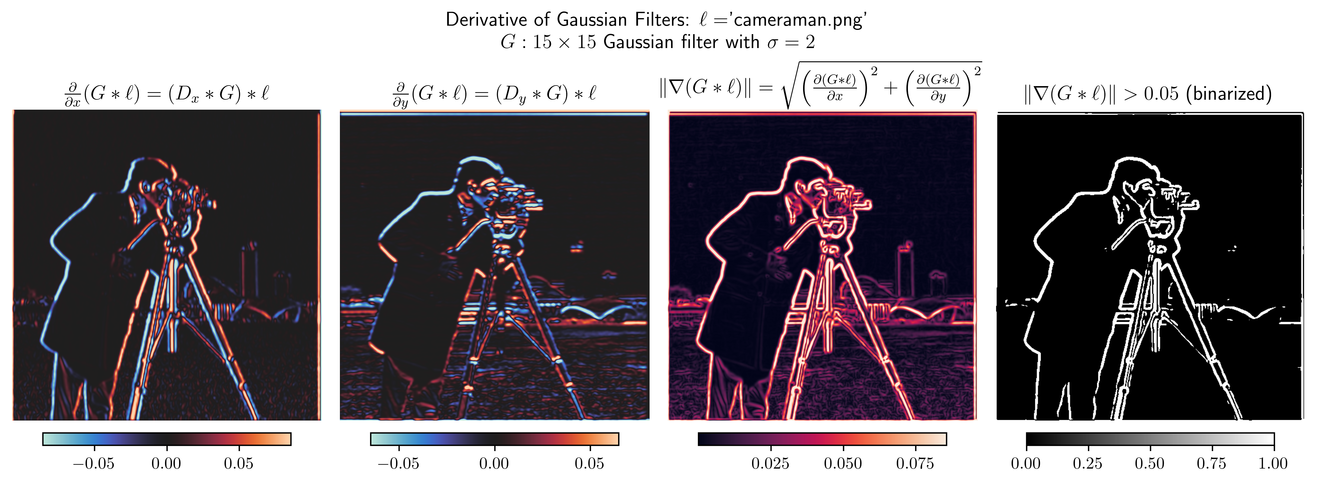
- Convolution with linear filters is well known to be an associative and commutative operation.
- Indeed, by comparing the two figures above verifies that convolving with a single filter and is equivalent to first convolving and , then convolving and .
- A similar equivalence holds for .

Part 2: Fun with Frequencies!
Part 2.1: Image "Sharpening"
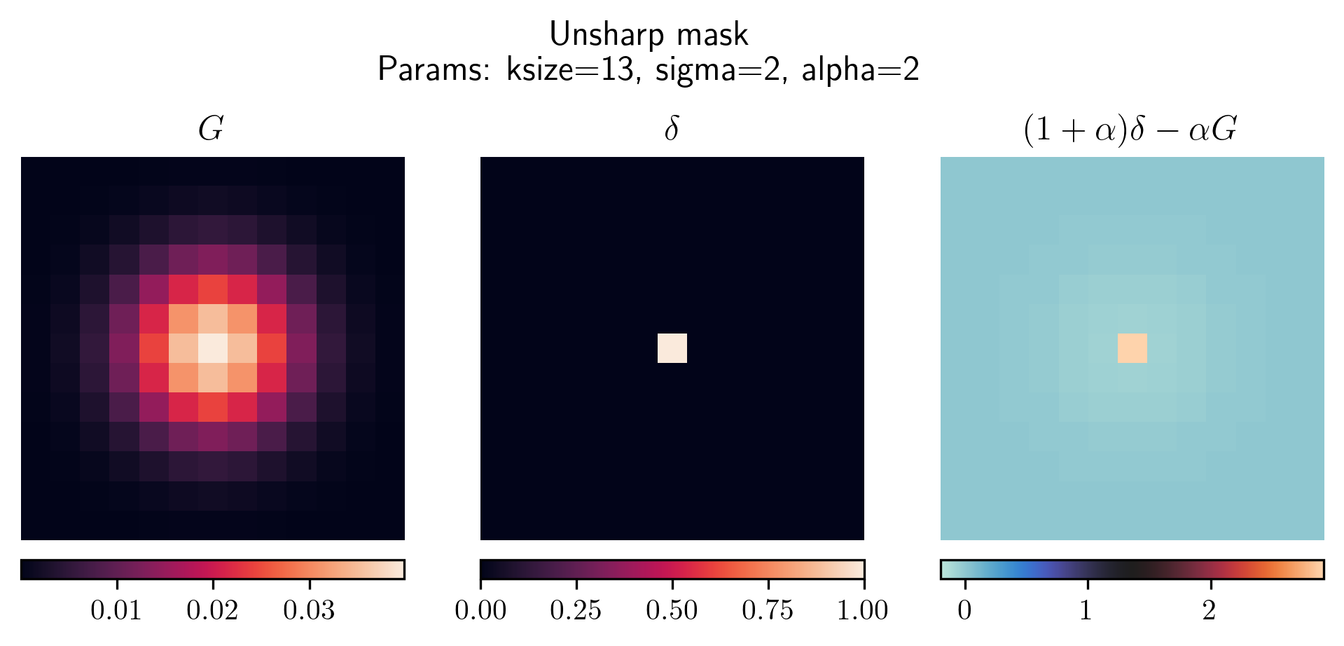
Let denote a given grayscale 2d image, denote the sharpening parameter, and denote a gaussian filter, and denote the unit impulse.
Starting from the given definition of the unsharp procedure, we apply the properties of convolution to simplify:
Hence, the unsharp filter can be applied with single convolution via .
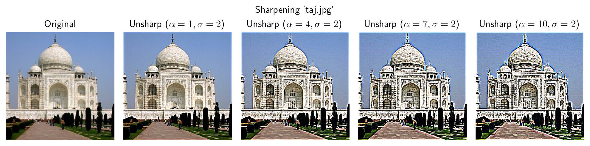
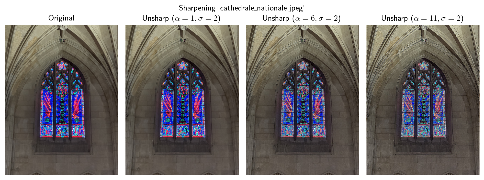
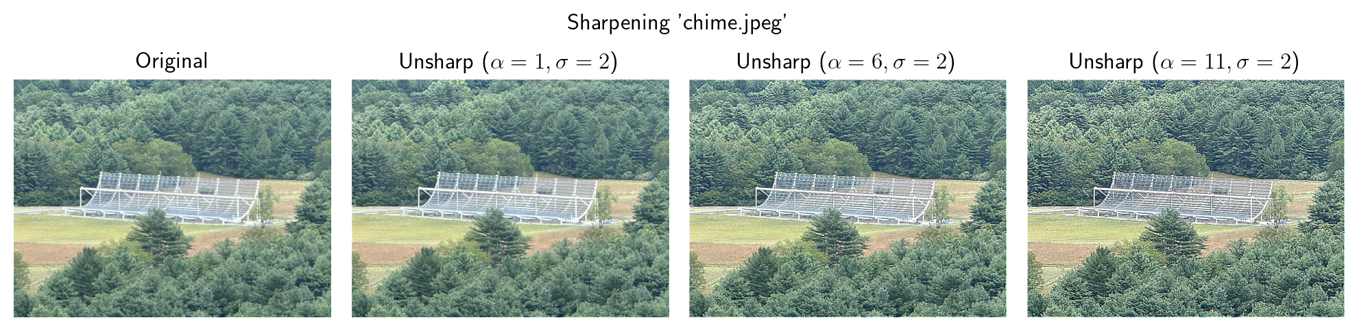
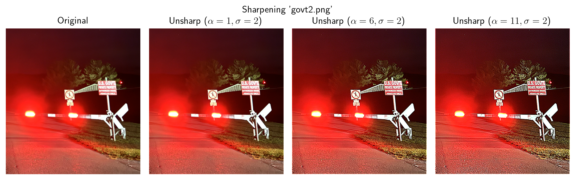
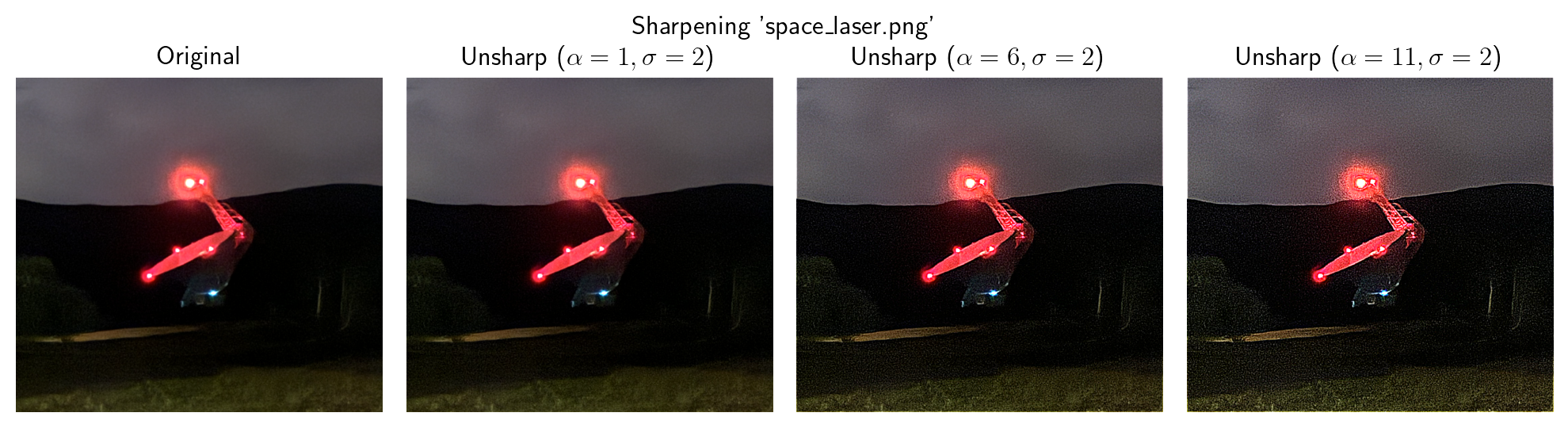
Experiment: Sharpen an Image, Blur It, then Sharpen It Again
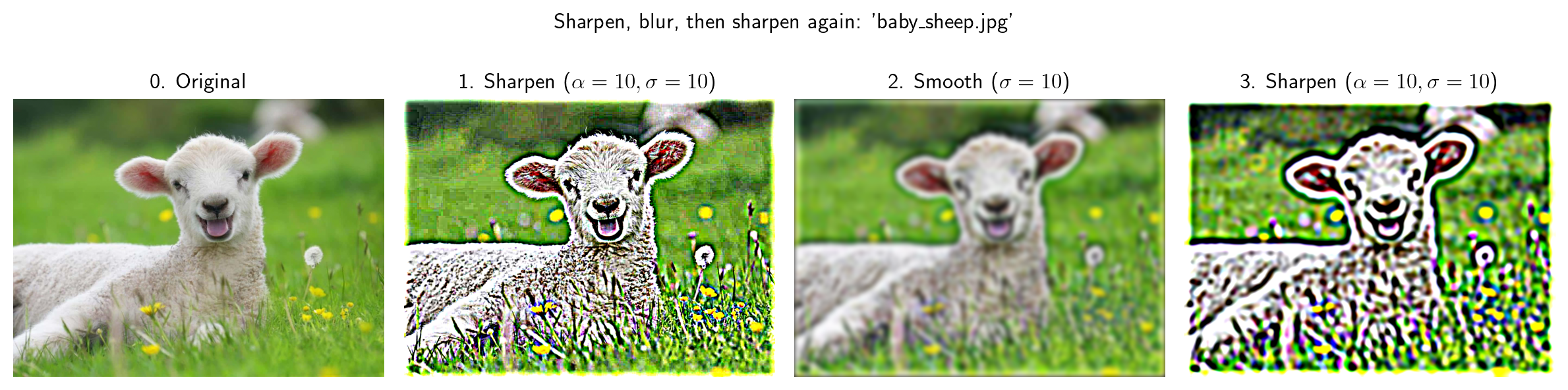
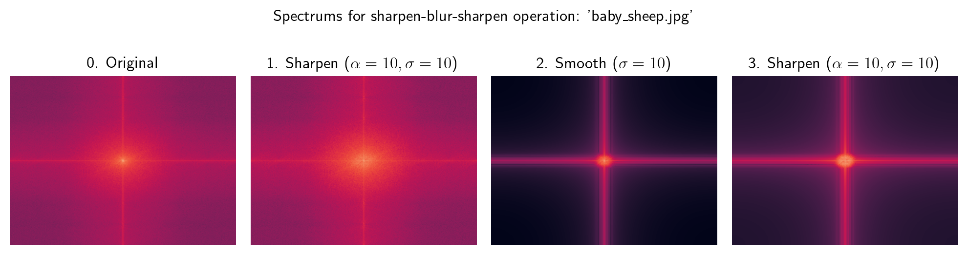
- Observations:
- First, the image and output of step 2 are not identical, so sharpen and smoothing operations with the same are not inverses.
- Further, as shown by the spectrums of these steps, the sharpen-blur-sharpen operation appears to be a lossy operation. This is true because step 2 low-passes the output of step 1 and heavily attenuates the high-frequency information present in the image.
- It appears that the high frequencies added by sharpening operation in step 3 are not enough to meaningfully undo this attenuation, so the final image contains most of the original low-frequency information but many artifacts from the unnaturally-enhanced high frequencies remaining after the low-pass operation.
Part 2.2: Hybrid Images
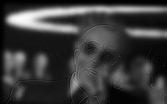
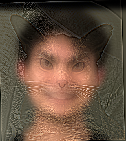


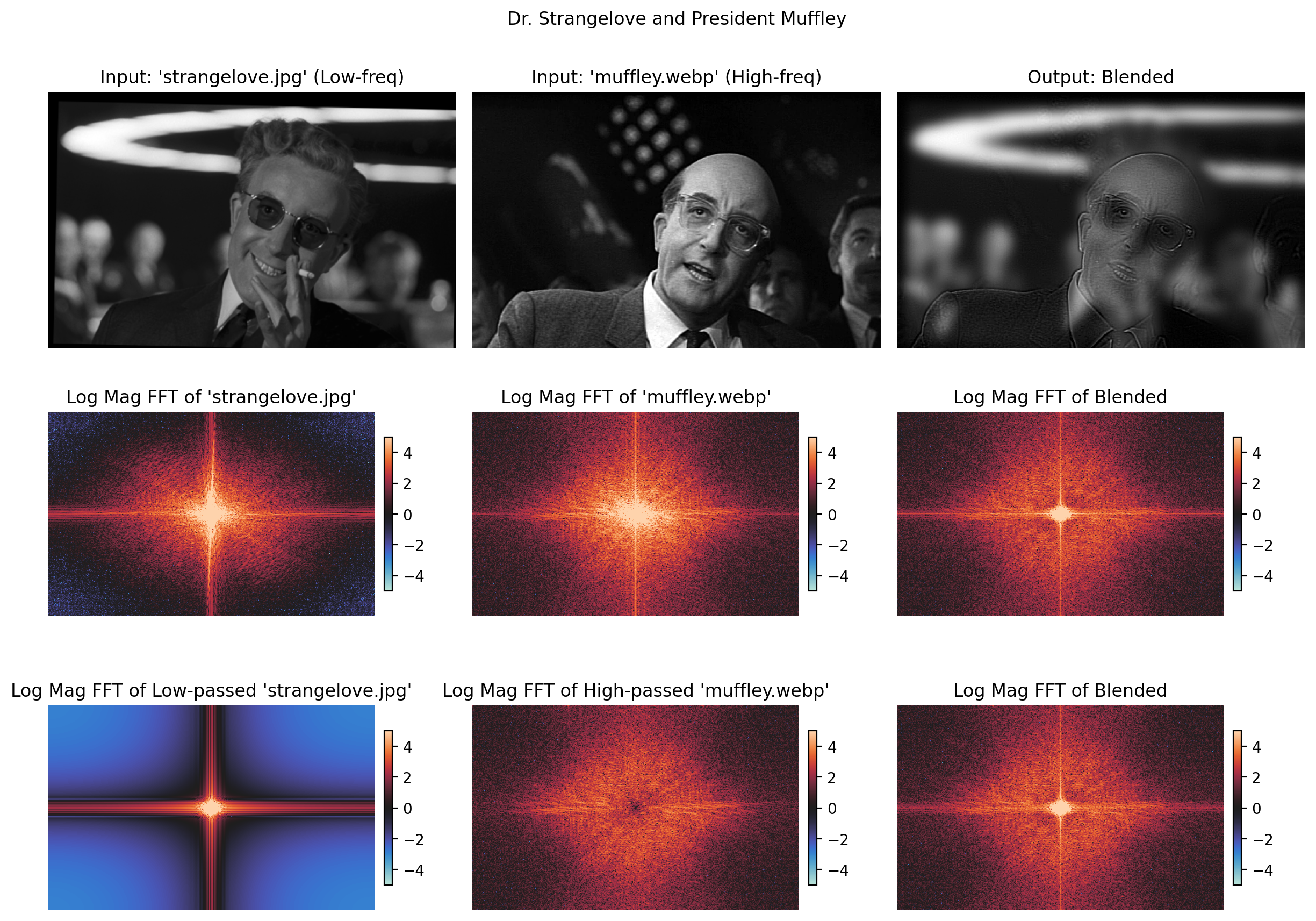
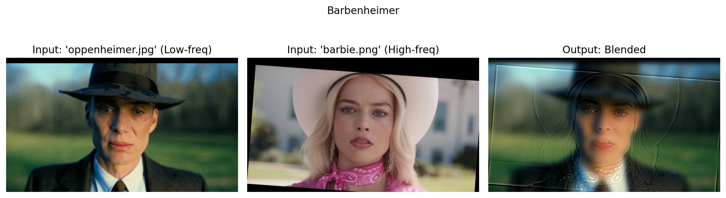
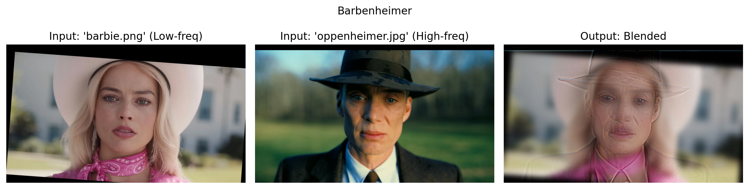
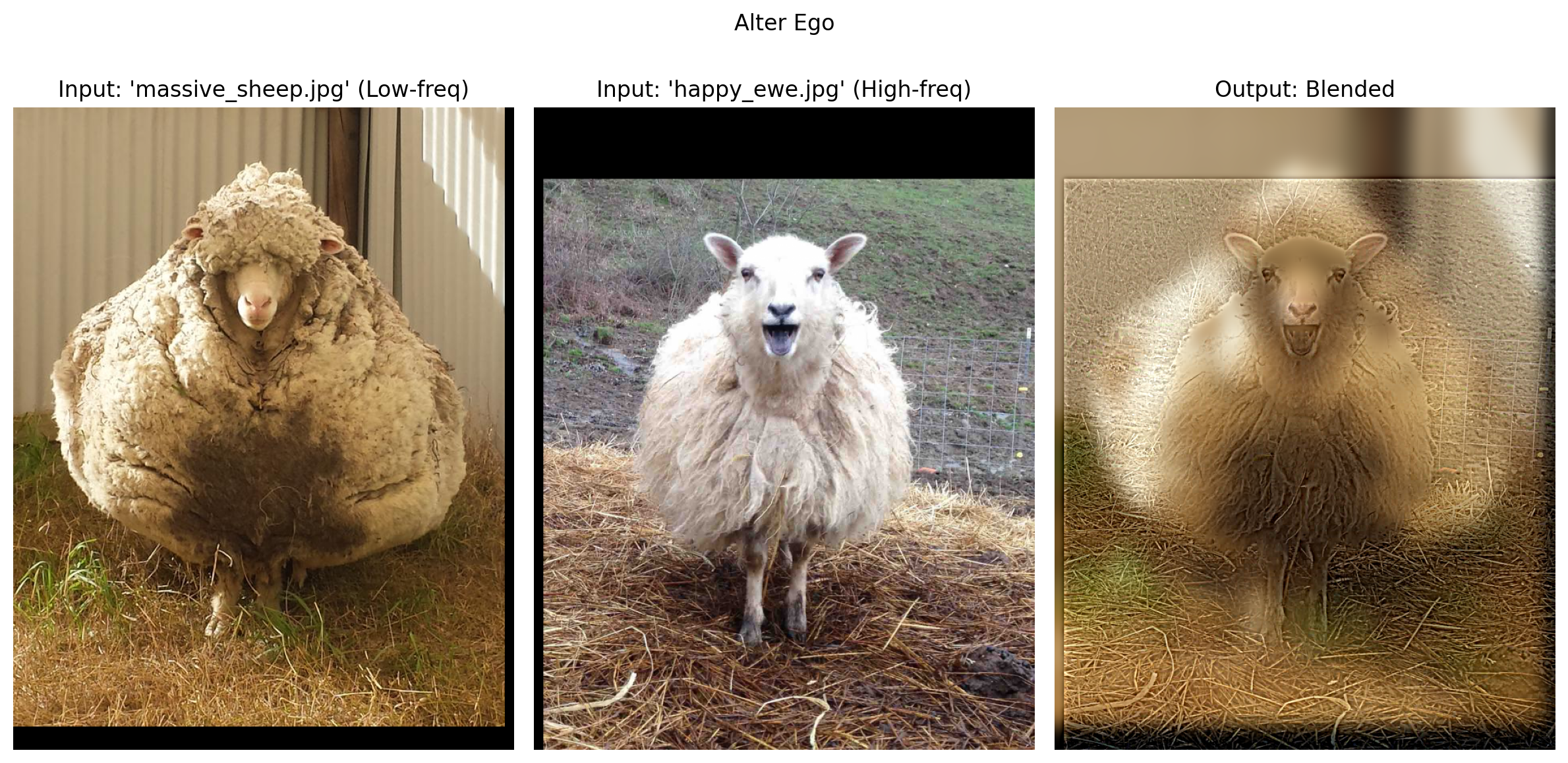
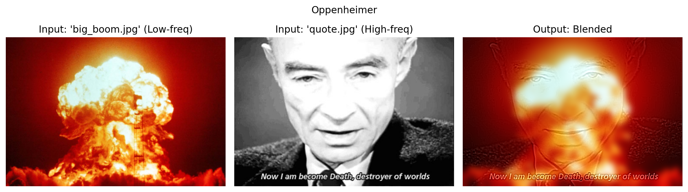
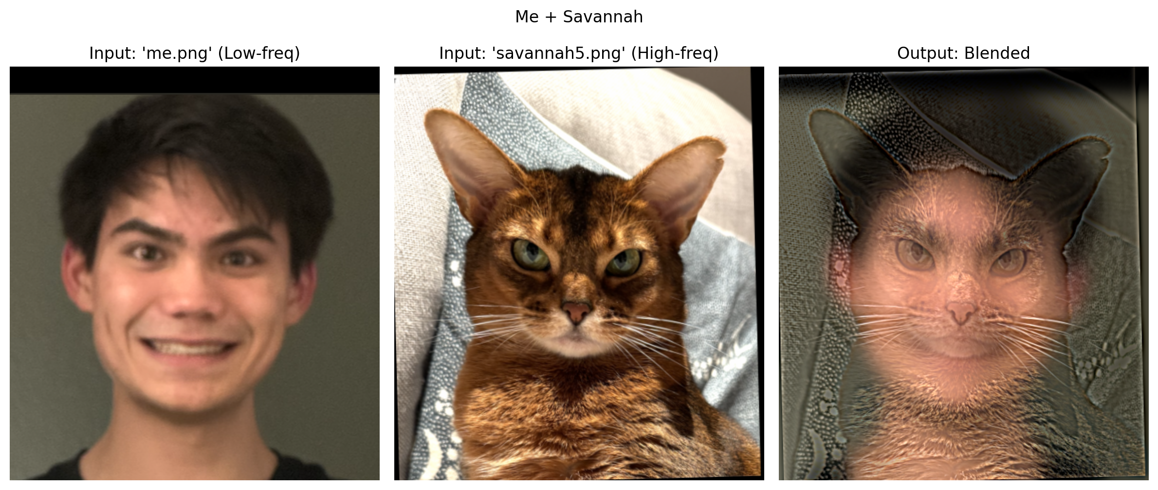
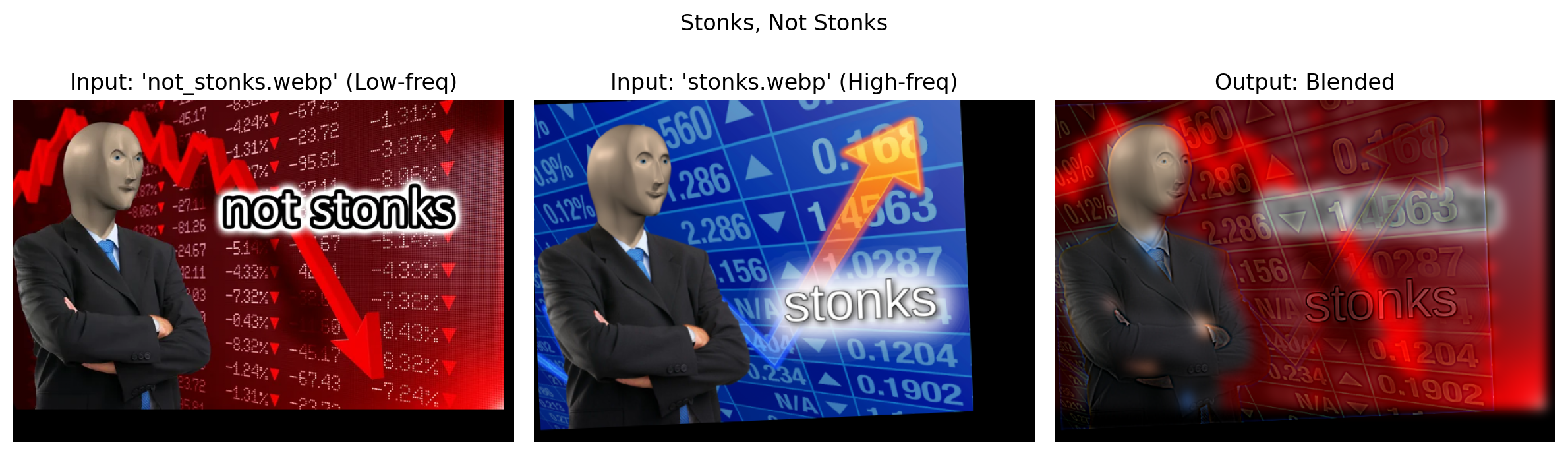
Input Images + Hybrid Result
Discussion: Colorizing Hybrid Images
- I experimented with adding color to my images to enhance the hybrid effect and, in all the image pairs I tried, the colors in the low-frequency image dominated the colors present in the hybrid image.
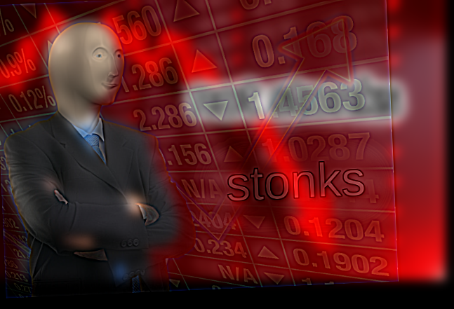
- The “Stonks, Not Stonks” hybrid (above) shows this phenomena quite clearly: the low-frequency component has a red background, the high-frequency component has a blue background, and the hybrid image has a red background.
- I think this happens because the background colors don’t change quickly and thus have their strongest components in low frequencies. As a result, color from the high-frequency component is hardly visible in the hybrid while color from the low-frequency component is visible at all distances in the hybrid, typically making the low-frequencies easier to see.
- Color tends to enhance perception of both high- and low-frequencies when the colors in both images align well, or at least don’t conflict.
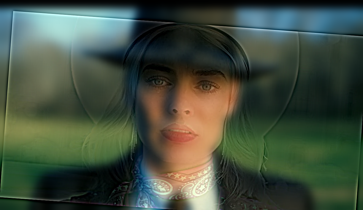
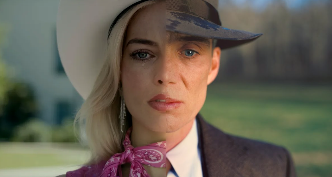
- For example, in our “Barbenheimer 2” the approximately-matching skin tones, common reddish/pinkish lip color, and gray/blue eyes, allow color in both low- and high-frequency components to enhance the hybrid effect at both scales.
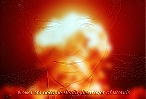
- As another example, consider “Oppenheimer”. Here, the fiery reds and oranges are highly visible at all distances and don’t really clash with the message and facial details in the colorless high-frequency component.
Barbenheimer 2 Oppenheimer
- When the colors don’t align well, color from the high-frequency component doesn’t have a significant impact on the hybrid, whereas adding color to the low-frequency component tends to make the hybrid better at far distances while worsening the high-frequency component at close distances.
- For example, in the “stonks, not stonks” hybrid, color seems to worsen the effect.
- At close distances, the red downwards-pointing arrow in the low-frequency is clearly visible at close distances and distracts from the upwards-pointing arrow in the high-frequency component.
Stonks, Not Stonks
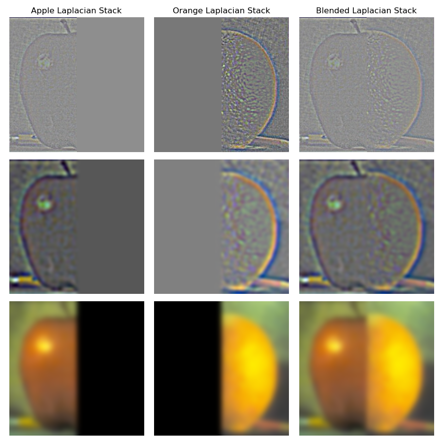
Part 2.3: Gaussian and Laplacian Stacks
Part 2.4: Multi-resolution Blending

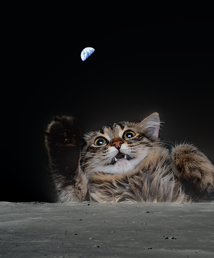
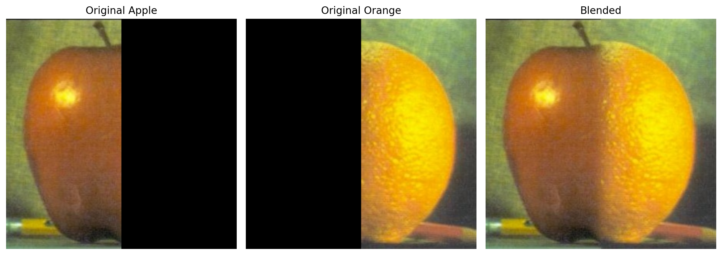
Input Images + Blended Result
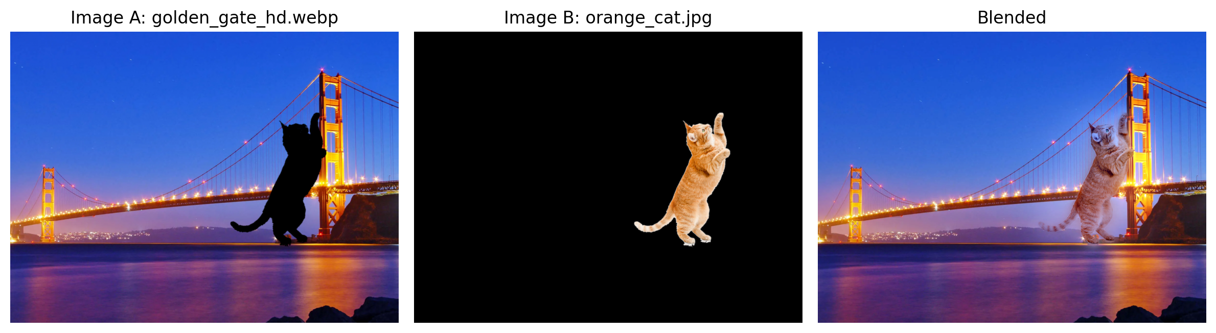

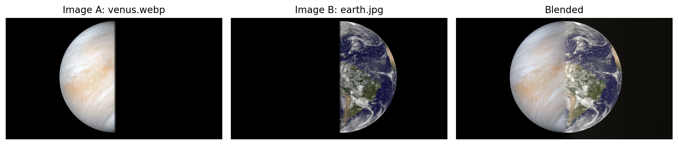
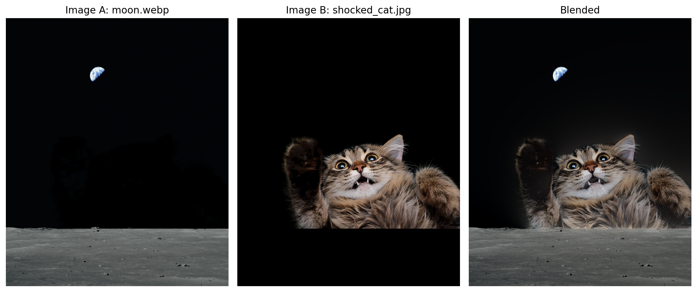
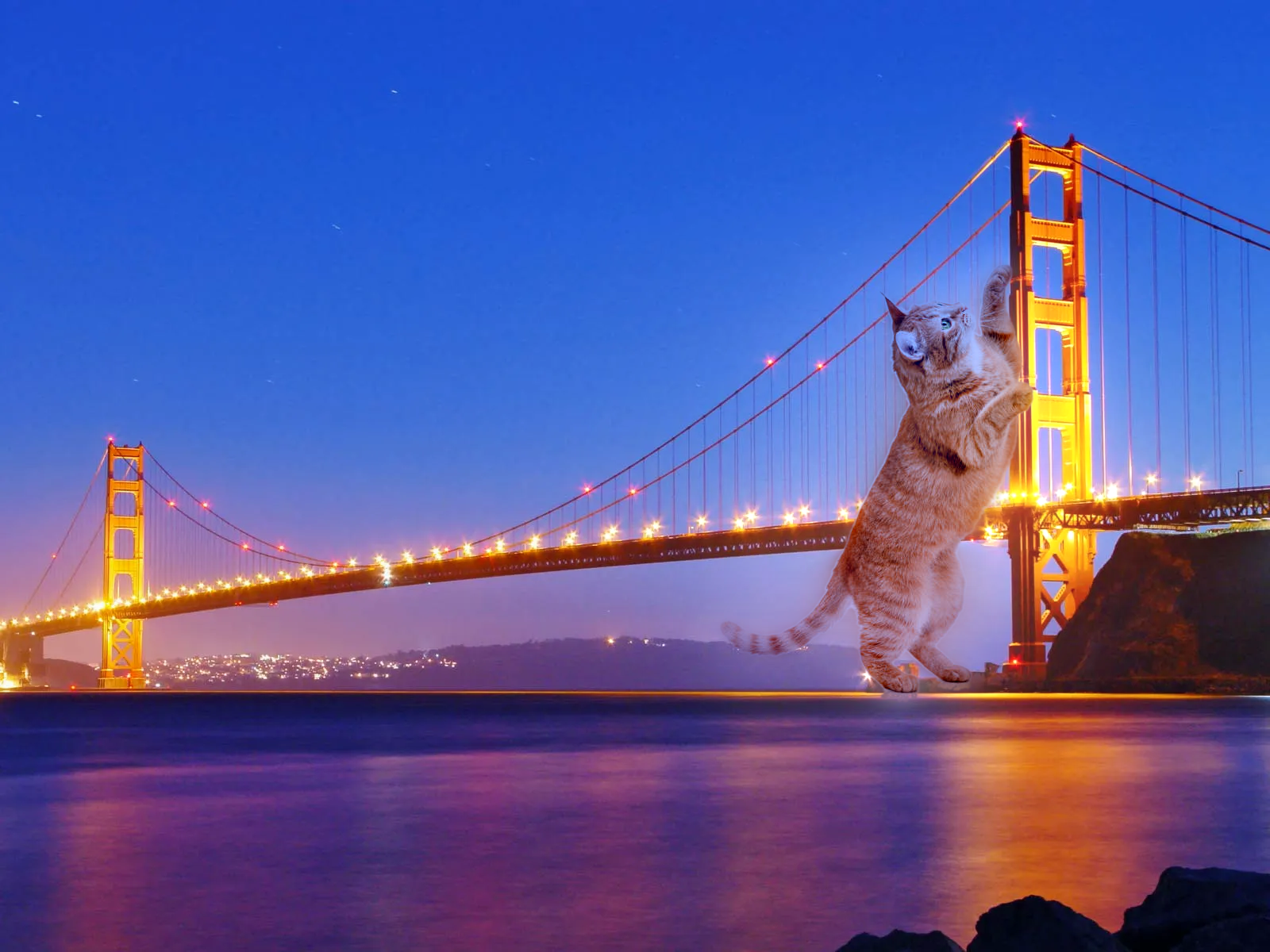
Discussion: Creating “Golden Gate Tabby“

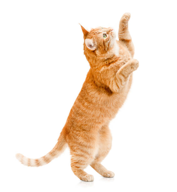
In this section, we’ll add an orange tabby cat to the Golden Gate Bridge to illustrate our process of blending two images together with an irregular mask.
Step 1: Select and Preprocess Images
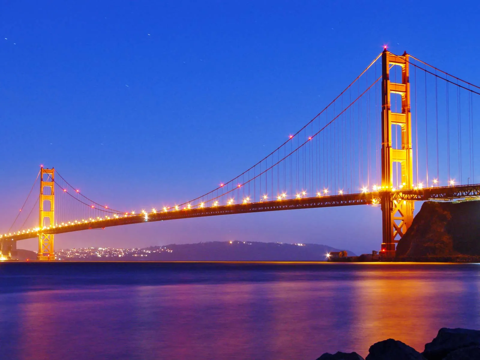
- Select a large image A to serve as the scene. In this case, A is a photo of the Golden Gate Bridge.
- Find a smaller image B satisfying the following conditions:
- B has dimensions no larger than A. (Cropping may be needed.)
- The subject in B can be easily separated from the background.
- Optionally crop or scale images A and B.
- Zero pad B to the dimensions of A.
- Use
np.rollto adjust the position of B on A until a good alignment is achieved.
- These adjustments can be fine-tuned by plotting , where is B after rolling.
- There will likely be an ugly rectangle around the object in image B that we will next remove in the next step.
Step 2: Create a Mask
- In this step, we’ll make a mask to extract the subject in B from its background.
- Select a threshold
- Our method for computing a good threshold involves computing statistics the maximum, minimum, sum, or mean of the color channel values at each pixel , then choosing a percentile cutoff of these values to serve as a binary threshold.
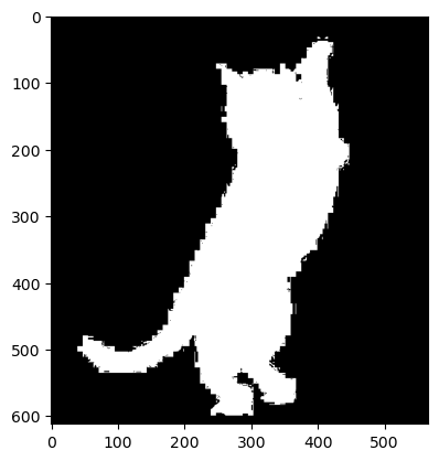
Mask with threshold set to 3 (pure white). 
Mask with threshold 2.94determined the 23rd percentile of color channel sums.
Mask with threshold 2.847determined the 23rd percentile of color channel maximums.
- Zero-pad the mask to the dimensions of A.
- Apply the same displacement found in step 1e to this mask.
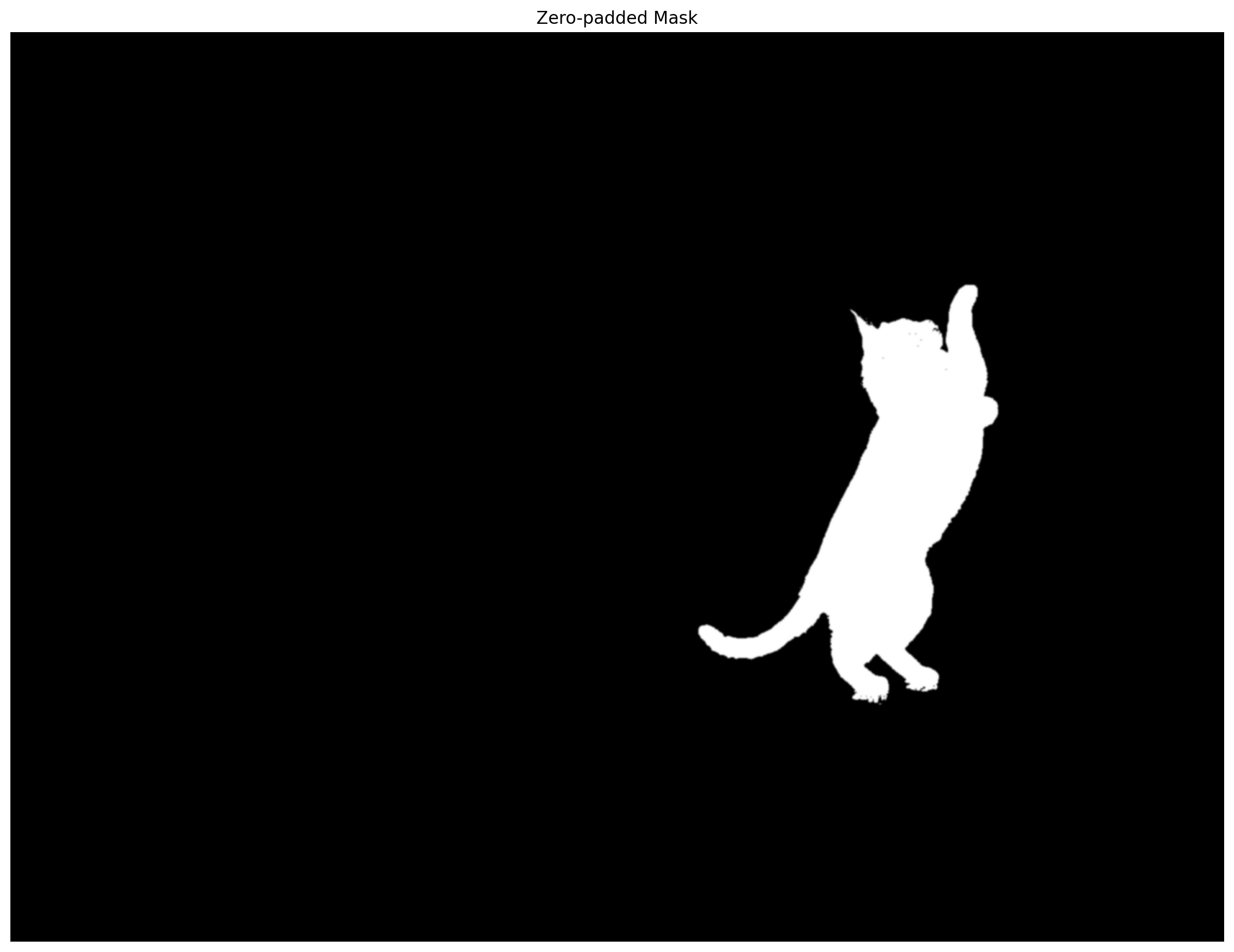
Step 3: Multi-resolution Blending
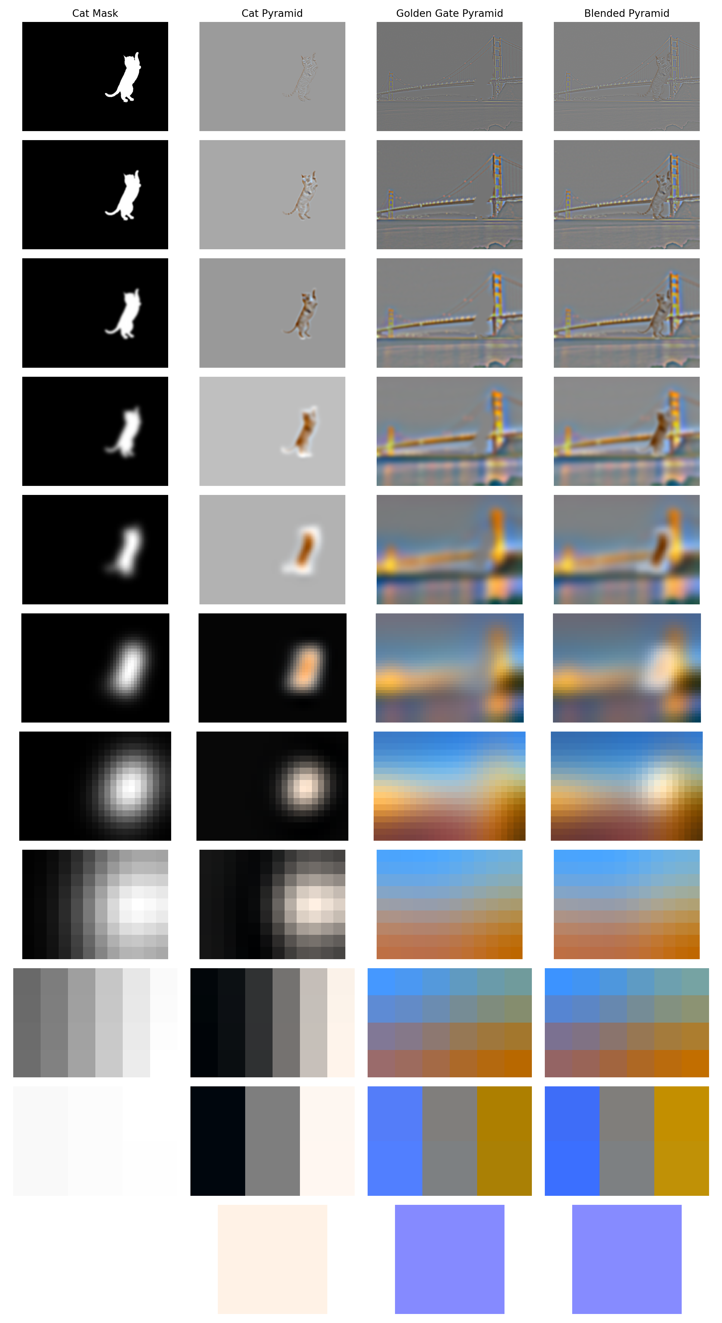
Apply the Laplacian blending method to blend Images A and B with our mask.
- Some experimentation is needed to find good parameters for the Gaussian smoothing and the depth of the Laplacian stack / pyramid.
What I Learned from This Project
This project taught me intuition about what 2D frequencies are and how they affect our perception of images. My work creating hybrid images was particularly enlightening because it gave me first-hand experience with human vision’s contrast-sensitivity curve: I could control the strength and believability of the hybrid effect just by adjusting the high- and low-frequency spectral content from each images.