CS180 Project 4A: Image Warping and Mosaicing

Author: Nicolas Rault-Wang (nraultwang at berkeley.edu)

Credit to Notion for this template.

1. Recovering a Homography

We begin by explaining how we estimate the homography transformation matrix $H$ to map $A$ into the geometry of $B$ .

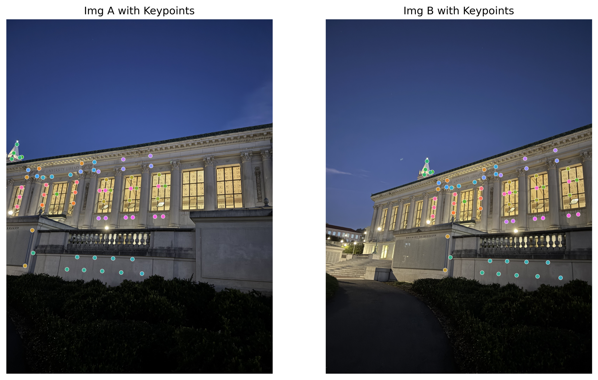
Two images $A$ and $B$ with the same center of projection are related by a homography. To estimate this transform, we first need to label a set of $N\geq 4$ feature correspondence points $(x_j, y_j) \leftrightarrow (x_j^\prime, y_j^\prime)$ between both images.

Note that $N$ must be at least 4 because homographies have 8 degrees of freedom due to scale invariance andeach pair of correspondences provides two constraints on $H$ .

1a. Establishing Point Correspondences

The figure below shows some example pairs of correspondence points. Well-defined edges are excellent features to correspond because they are easy to identify in both images.

1b. Estimating the Homography

While a minimum of 4 correspondence pairs are required to solve for $H$ , this system is very sensitive to noise. To produce a more robust homography, we use more than 4 correspondence pairs to form an over-determined system, then use least-squares to obtain an estimate of the free parameters of $H$ .

Working in homogeneous coordinates, the derivation of two equations constraining the free parameters of $H$ from an arbitrary correspondence pair $(x_j, y_j) \leftrightarrow (x_j^\prime, y_j^\prime)$ is straightforward:

\begin{bmatrix}a&b&c\\d&e&f\\g&h&1\end{bmatrix}\begin{bmatrix}x_j\\y_j\\1\end{bmatrix} = w \begin{bmatrix}x_j^\prime\\y_j^\prime\\1\end{bmatrix}

\begin{cases}ax_j + by_j + c &= wx_j^\prime\\dx_j + ey_j + f &= wy_j^\prime\\gx_j + hy_j + 1 &= w\end{cases} \implies \begin{cases}ax_j + by_j + c &= (gx_j + hy_j + 1) x_j^\prime \\ dx_j + ey_j + f &= (gx_j + hy_j + 1) y_j^\prime \end{cases}

\begin{cases} ax_j + by_j + c +0d+0e+0f- gx_j x_j^\prime - hy_j x_j^\prime = x_j^\prime \\ 0a + 0b + 0c +dx_j + ey_j + f - gx_j y_j^\prime - hy_j y_j^\prime = y_j^\prime \end{cases}

Stacking all $2N$ equations into an $2N\times 8$ feature matrix $X$ and $2N\times 1$ target vector $\vec y$ gives

\underbrace{\begin{bmatrix}x_1&y_1&1&0&0&0&-x_1x_1^\prime&-y_1x_1^\prime \\0&0&0&x_1&y_1&1&-x_1y_1^\prime&-y_1y_1^\prime\\&&&&\vdots&&&&\\x_j&y_j&1&0&0&0&-x_jx_j^\prime&-y_jx_j^\prime \\0&0&0&x_j&y_j&1&-x_jy_j^\prime&-y_jy_j^\prime\\&&&&\vdots&&&&\\x_N&y_N&1&0&0&0&-x_Nx_N^\prime&-y_Nx_N^\prime \\0&0&0&x_N&y_N&1&-x_Ny_N^\prime&-y_Ny_N^\prime \end{bmatrix}}_{X} \vec \theta= \underbrace{\begin{bmatrix} x_1^\prime \\ y_1^\prime\\\vdots\\x_j^\prime \\ y_j^\prime\\\vdots\\x_N^\prime \\ y_N^\prime\end{bmatrix}}_{\vec y}

where we have unrolled $H$ into $\vec \theta = \begin{bmatrix}a&b&c&d&e&f&g&h\end{bmatrix}^T$ .

For $N \geq 4$ well-chosen correspondence points $(x_j, y_j) \leftrightarrow (x_j^\prime, y_j^\prime)$ , the columns of $X$ are linearly independent, making $X$ have full column rank. Hence, the least-squares estimate of $\vec\theta$ , and thus $H$ , is uniquely given by

\vec\theta^* = (X^TX)^{-1}X^T\vec y

2. Warping Images with a Homography

In all following sections, we’ll use the term “canvas” to refer to an $xy$ -axis aligned bounding box that is large enough to contain all points in the image of the homography transform.

2a. Warping One Image

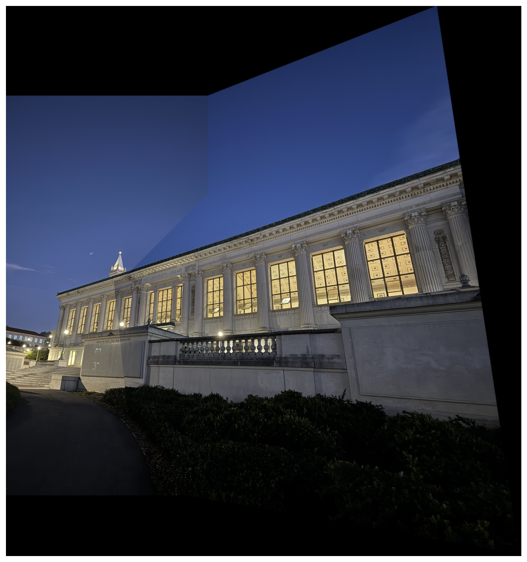
With the homography $H$ relating $A$ and $B$ , we map $A$ into $B$ with an inverse warping procedure:

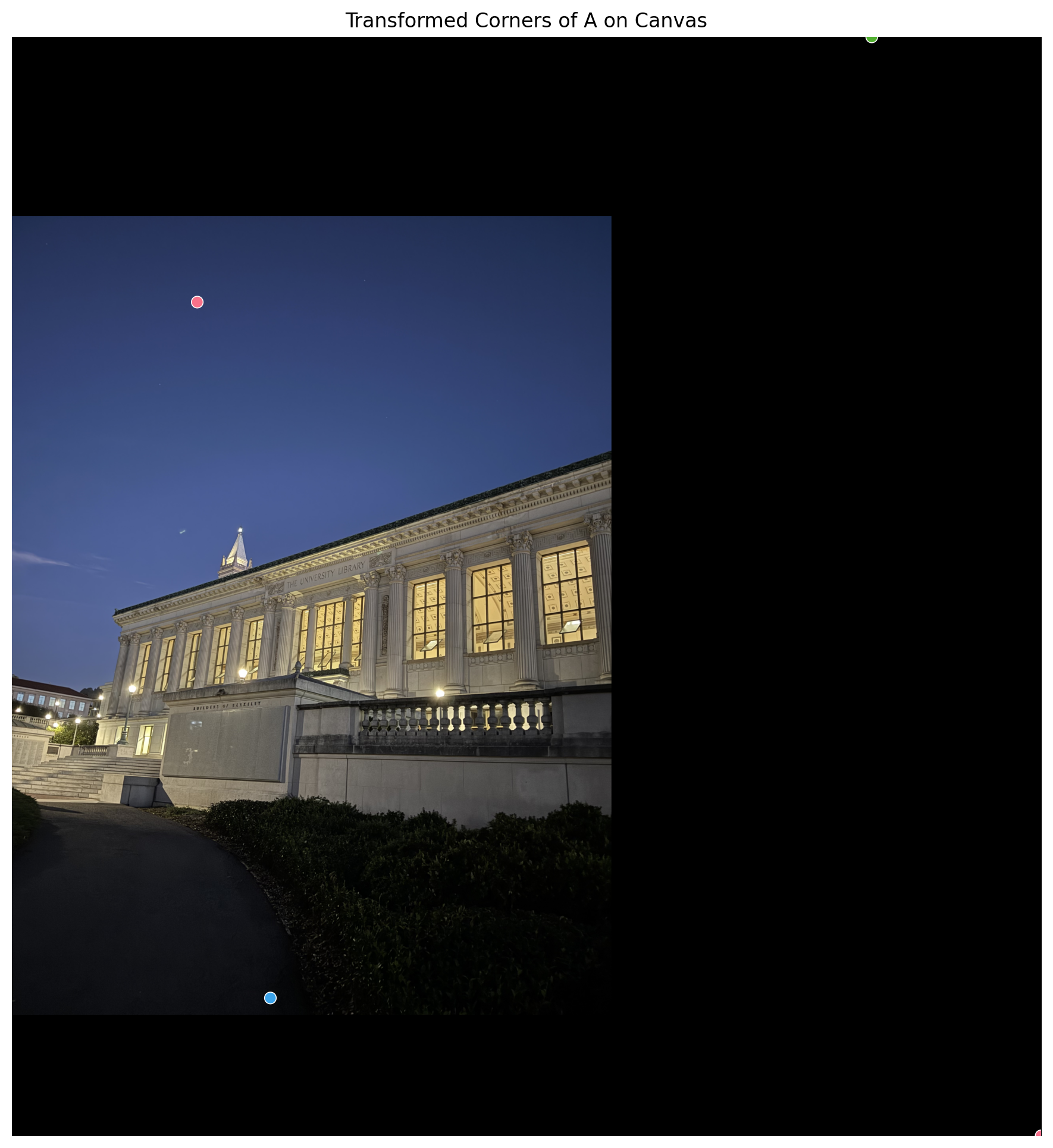
Determine the minimum dimensions of the canvas by warping the corners of $A$ into $B$ .

For every canvas pixel $(i^\prime, j^\prime)$ in the quadrilateral formed from the warped corners of $A$ , compute the point $(x,y)$ in the geometry of $A$ by inverting the homography.
$\begin{bmatrix}x \\y\\1\end{bmatrix} = H^{-1}\begin{bmatrix}i^\prime \\j^\prime\\1\end{bmatrix}$

In general, $(x,y)$ will not lie exactly on a grid point in $A$ , so we interpolate the RGBA color vector $C(i^\prime, j^\prime)$ at $(x,y)$ from the grid points of $A$ . Our code uses scipy.interpolate.RegularGridInterpolator to do this.

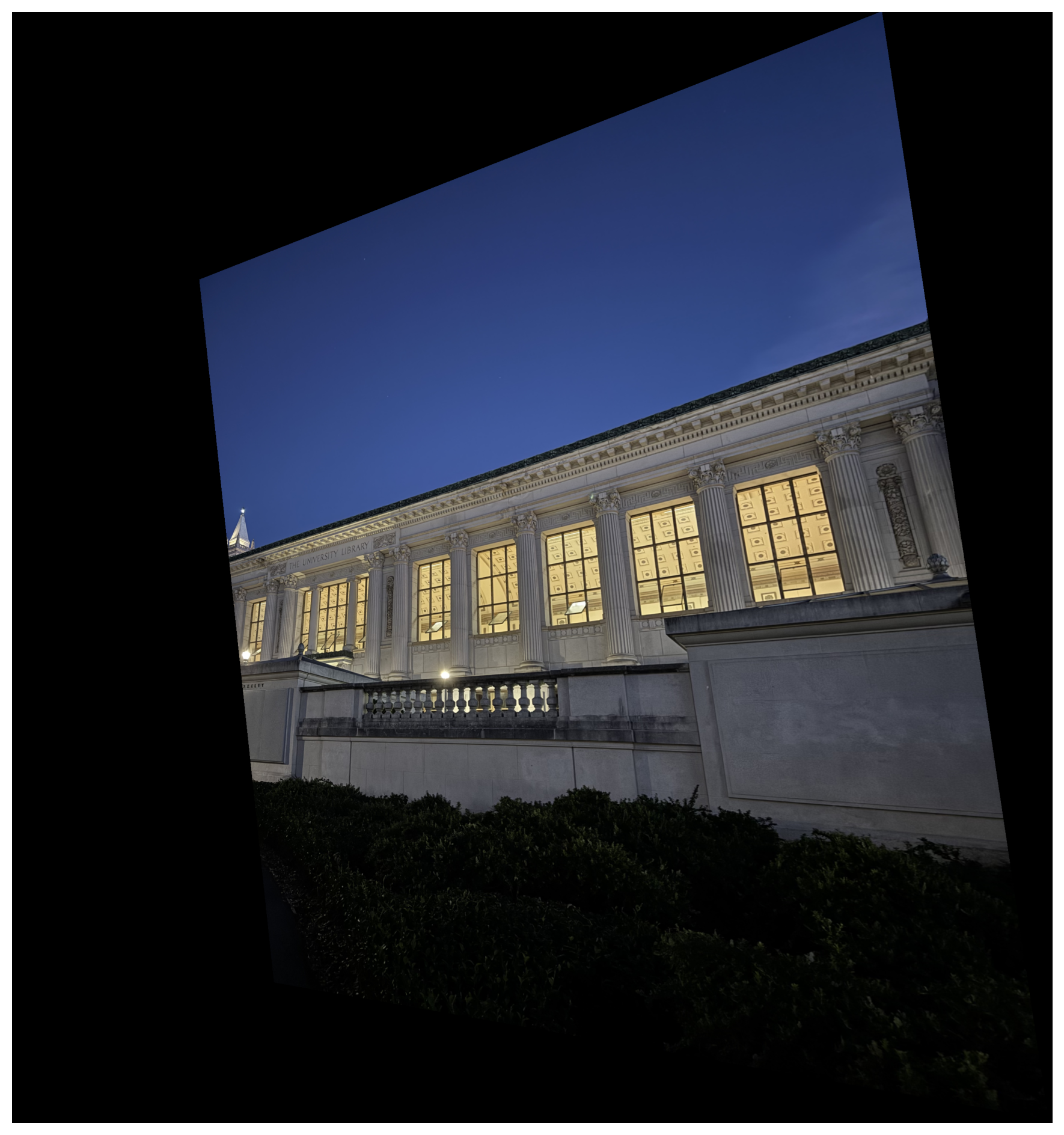
After completing steps 2 and 3, we have the color value $C(i^\prime, j^\prime)$ at each canvas point $(i^\prime, j^\prime)$ , completing the process of inverse-warping $A$ to the canvas with $B$ , producing $A^\prime$ in the geometry of $B$ .

To avoid edge-artifacts, we use a 2-level laplacian pyramid to smoothly blend $A^\prime$ and $B$ .
1. We found that a mask created from the Euclidean distance transform on $A^\prime$ and $B$ works very well. Our code uses scipy.ndimage.distance_transform_edt to do this.

The canvas is computed by transforming the corners of $A$ with the homography $H$ .

$A^\prime$ : the result of warping $A$ into the common canvas via the homography $H$ .

2b. Image Rectification

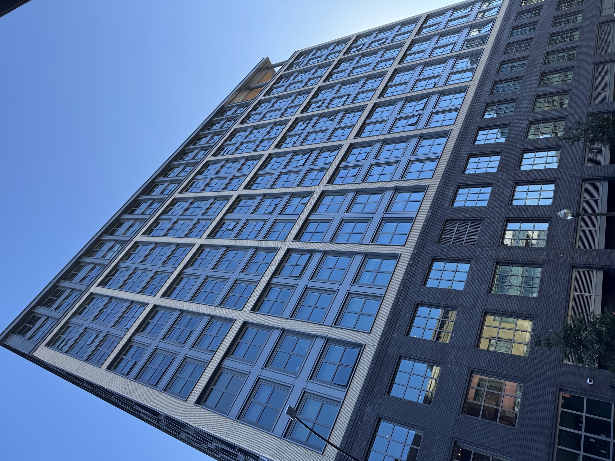
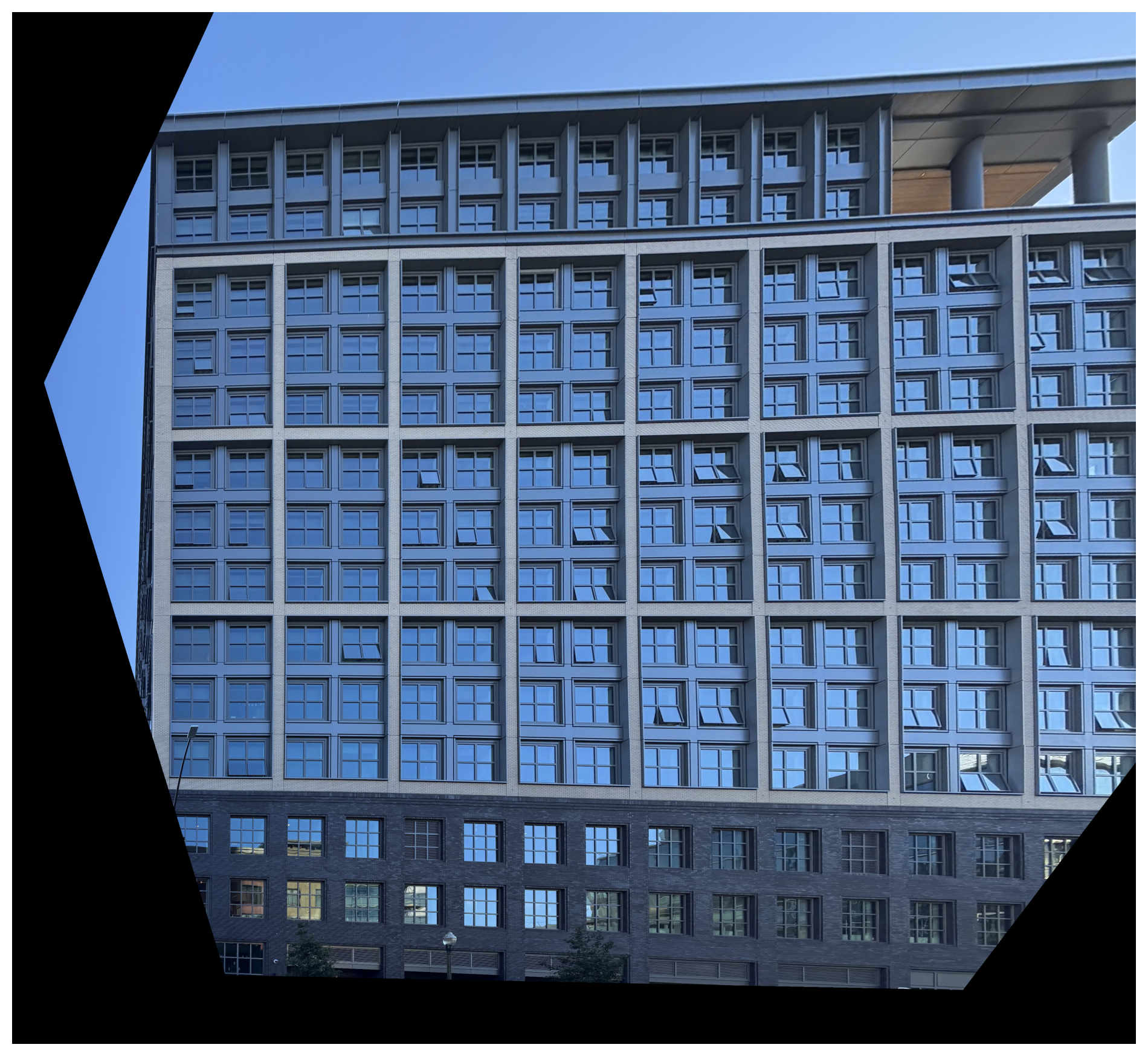
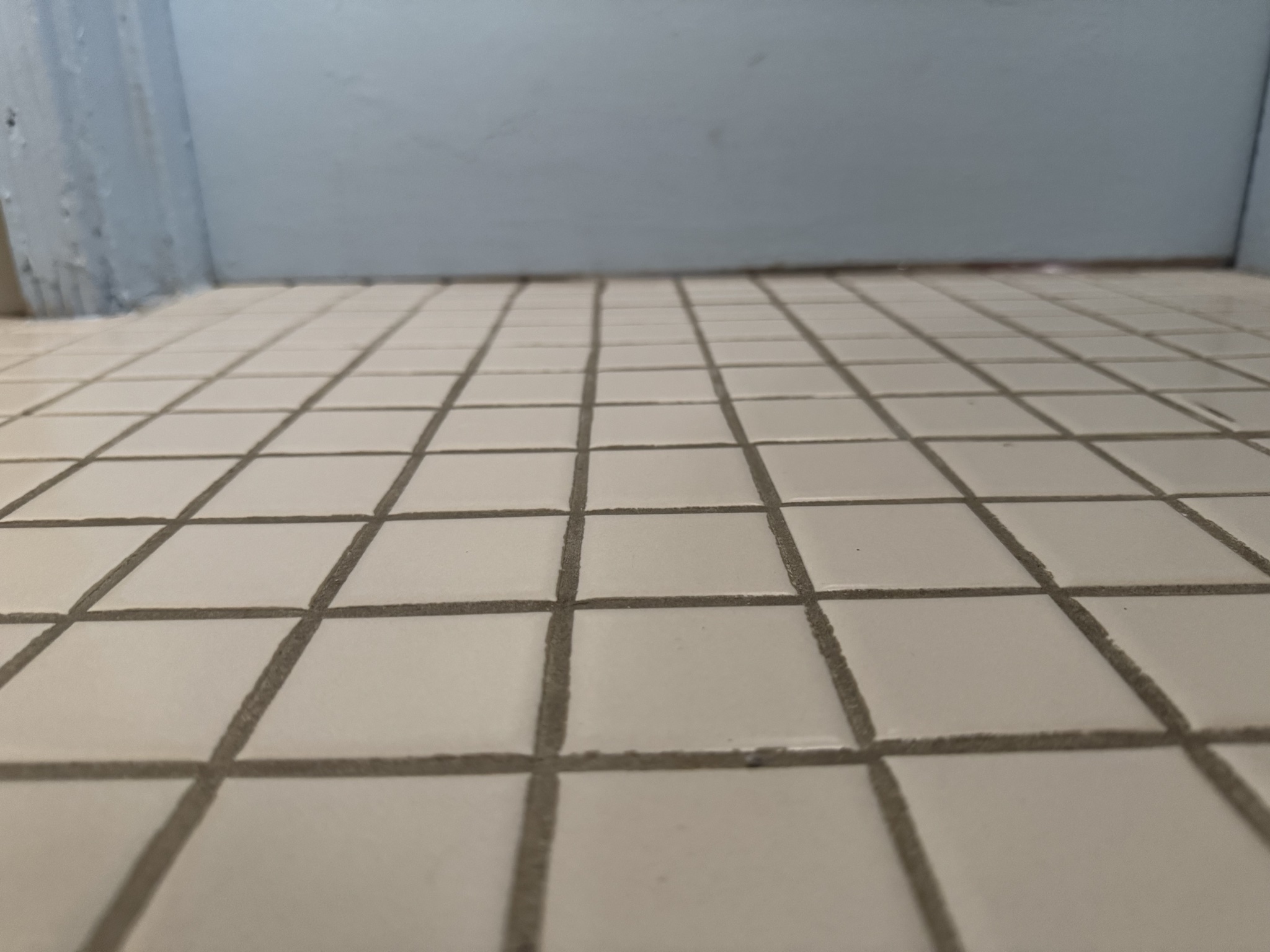
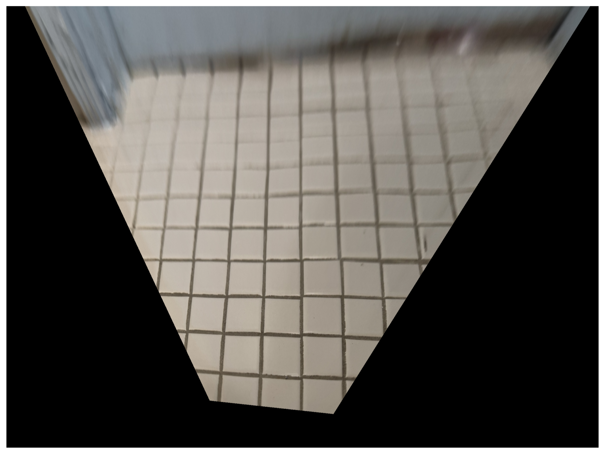
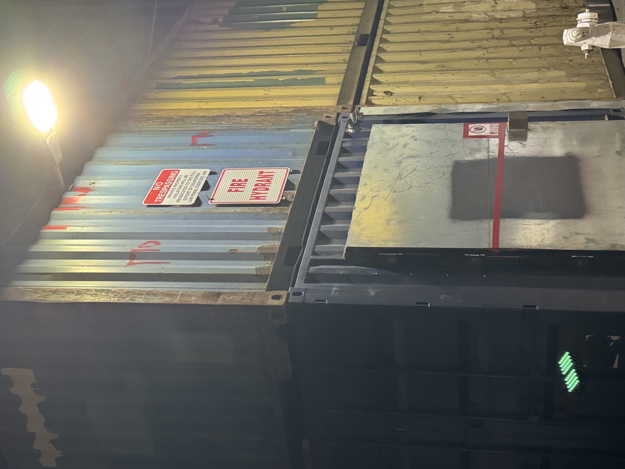
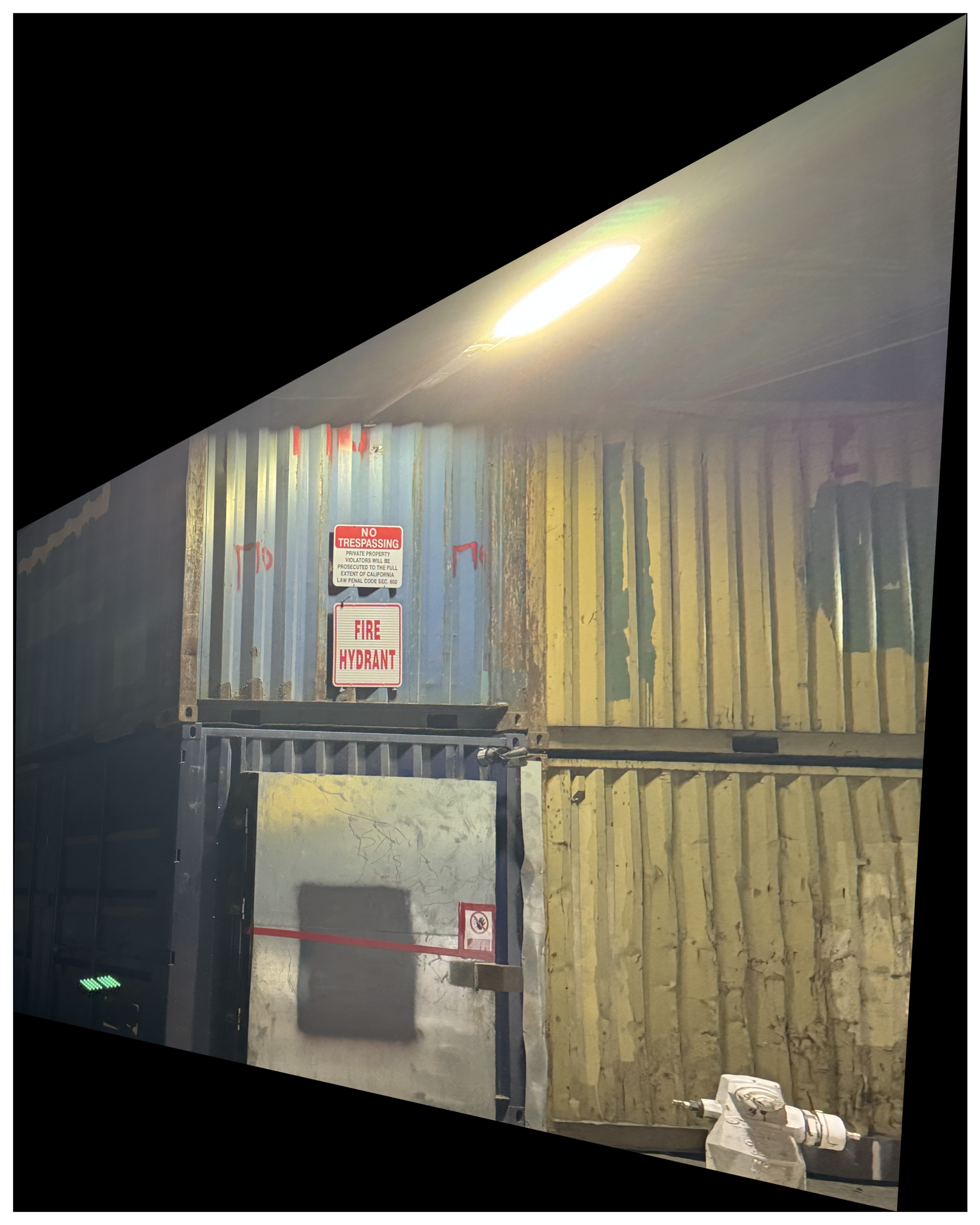
An application of homography warping is undoing (rectifying) the perspective distortion of rectangular objects in images. This is theoretically possible because two images of a planar rectangular-looking object, like a tile or poster, are related by a homography.

Below, we show some examples of this operation. The image on the left is the original and the image on the right is the result of rectification.

Rectification of the rectangular windows of the building.

Rectification of the bathroom floor tiles.

3. Creating Panoramas

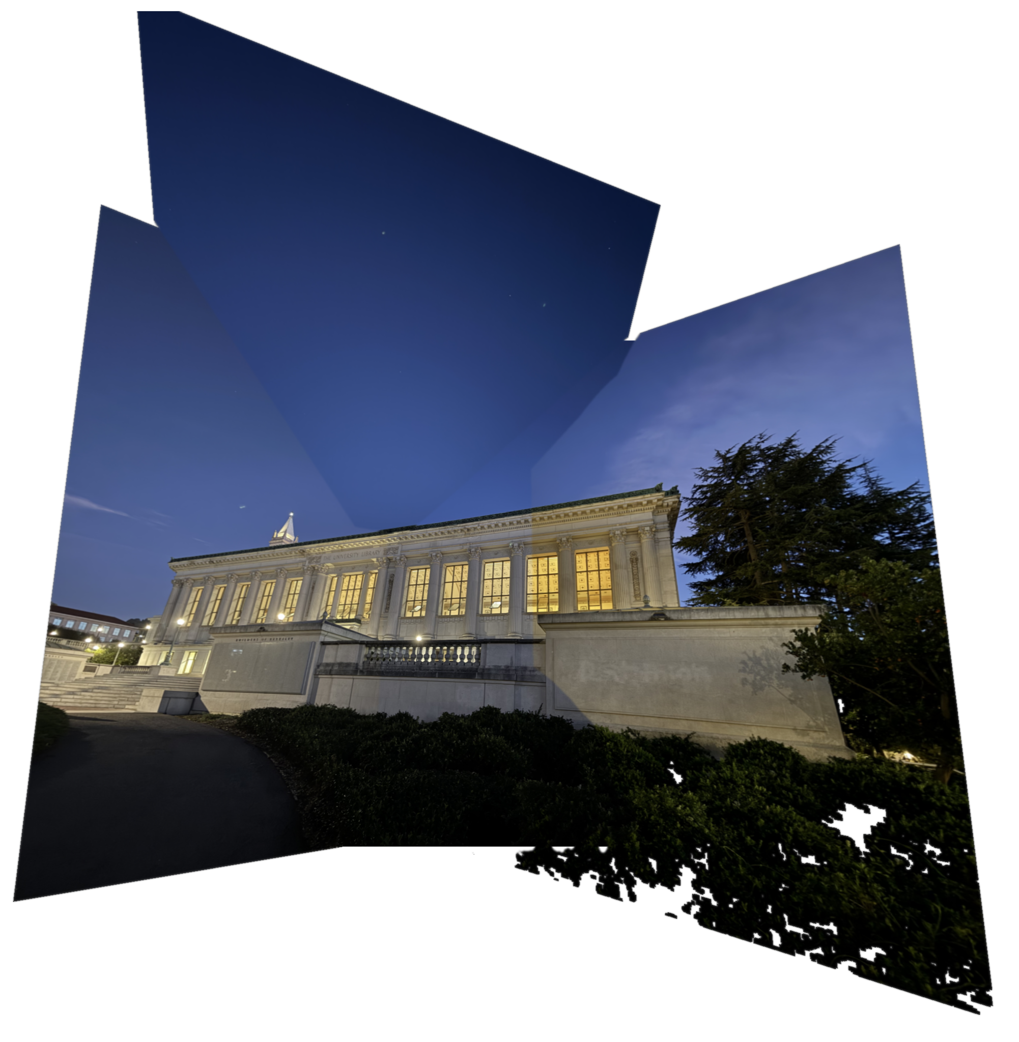
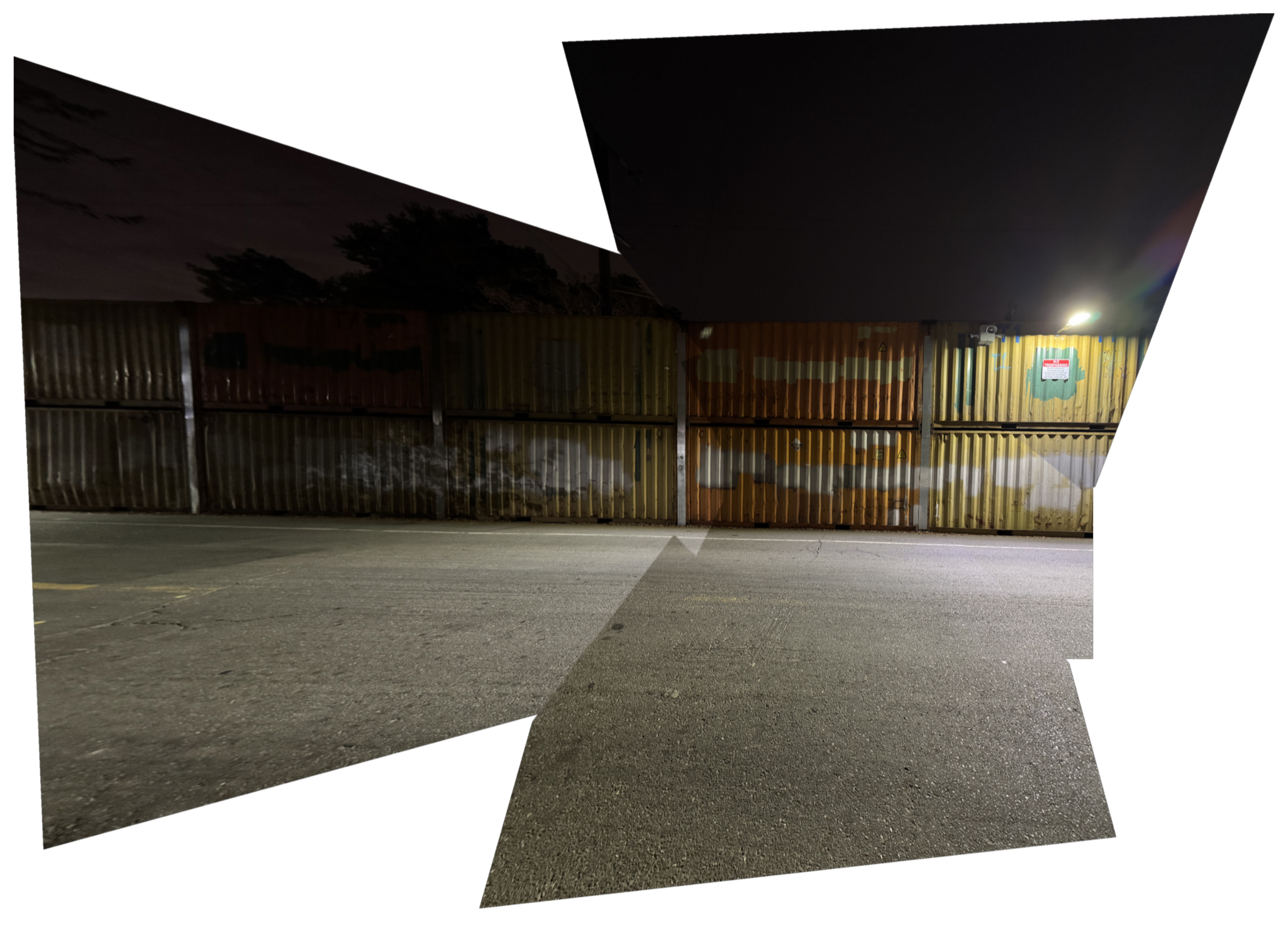
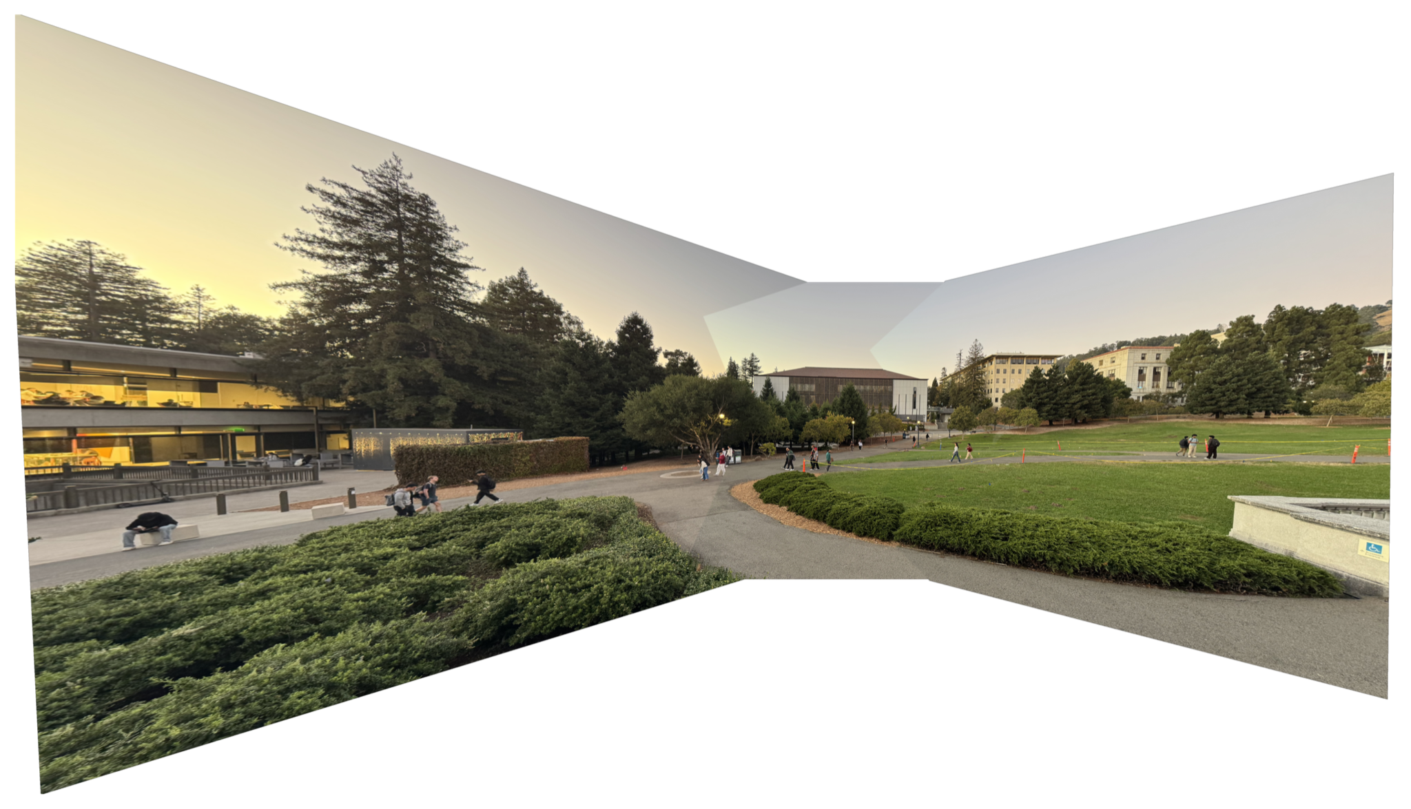
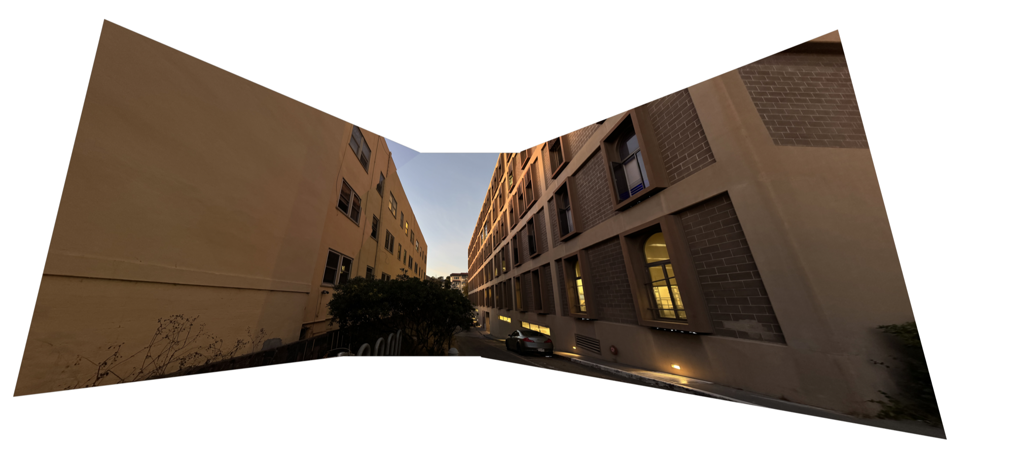
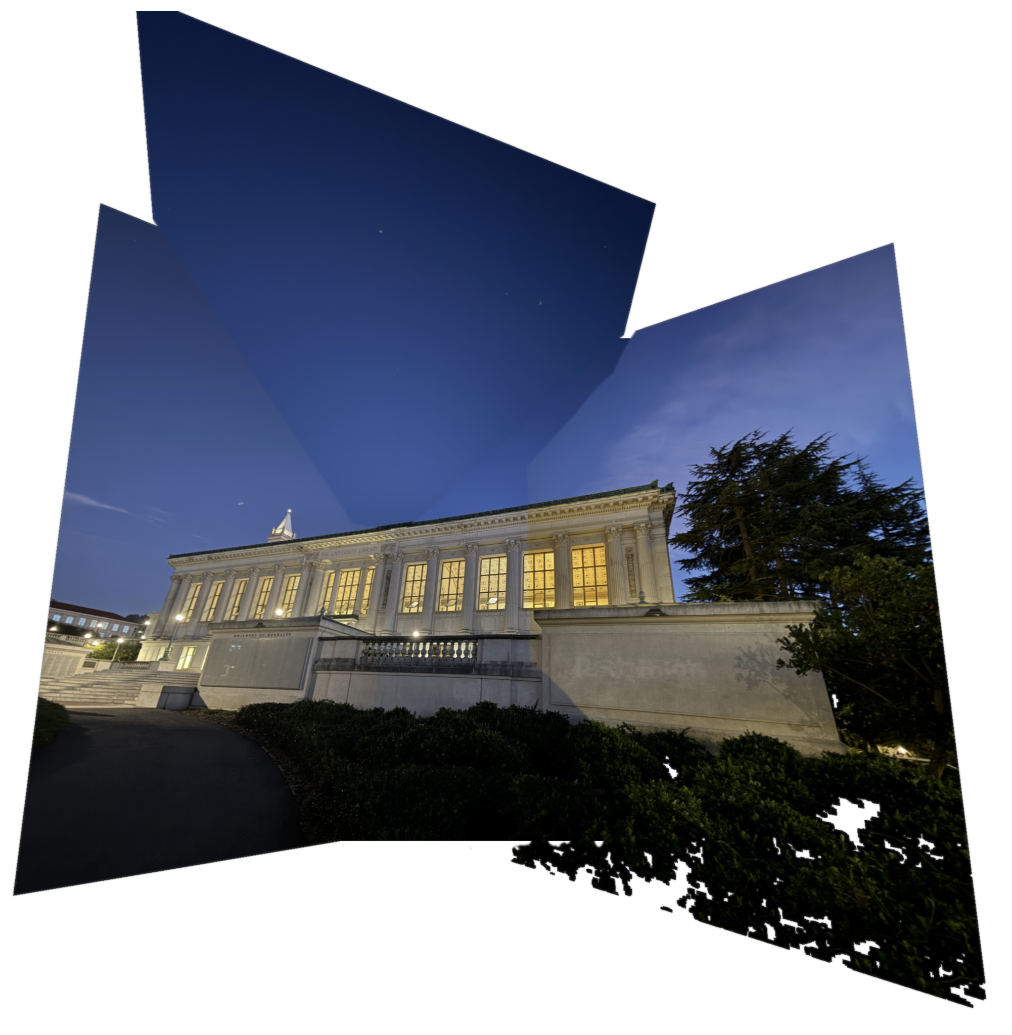
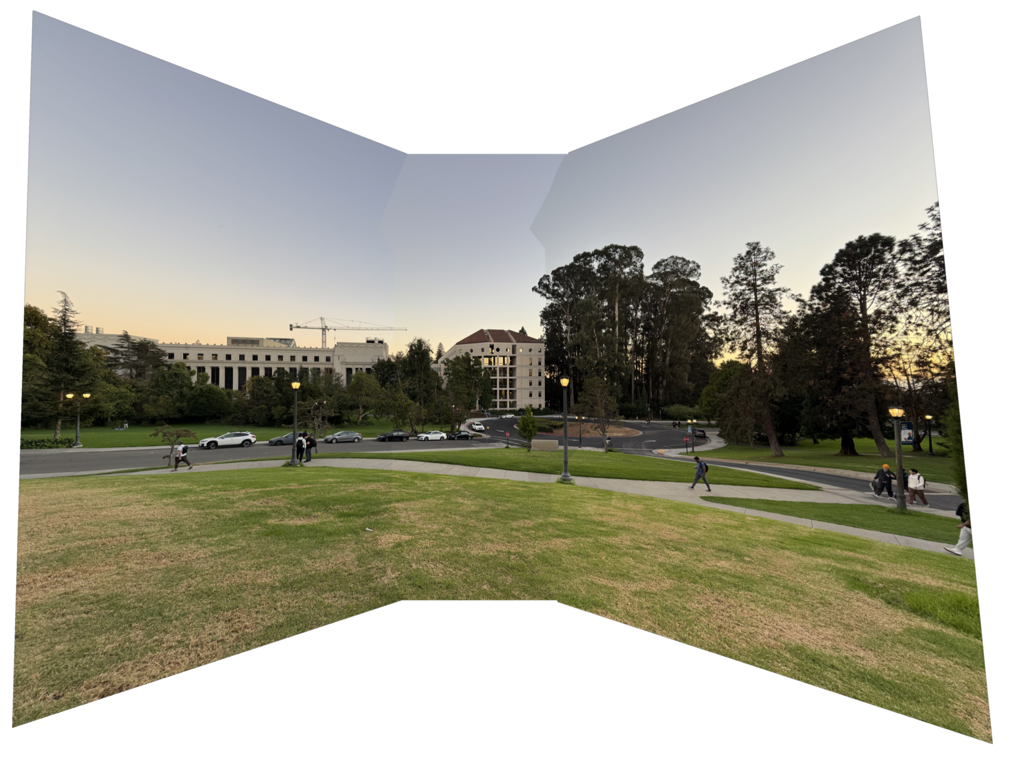
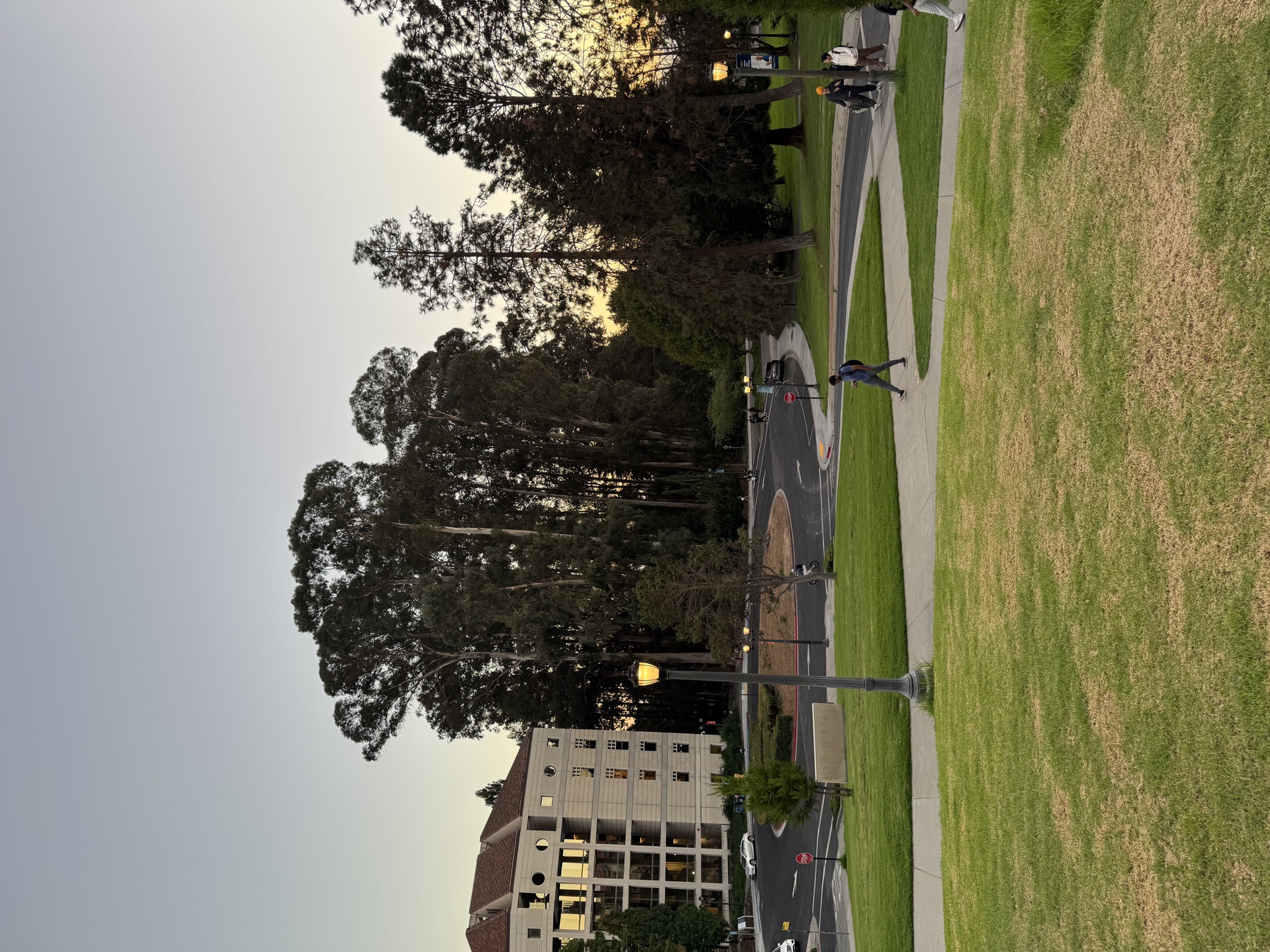
We can extend our one-image warping procedure to create panoramas. Since two images with the same center of projection are related by a homography, we can form a panorama by warping a set of images with the same center of projection into a particular image in this set. This can be implemented by recursively applying the the one-image warp to grow a panorama one image at a time.

3a. Panorama Examples

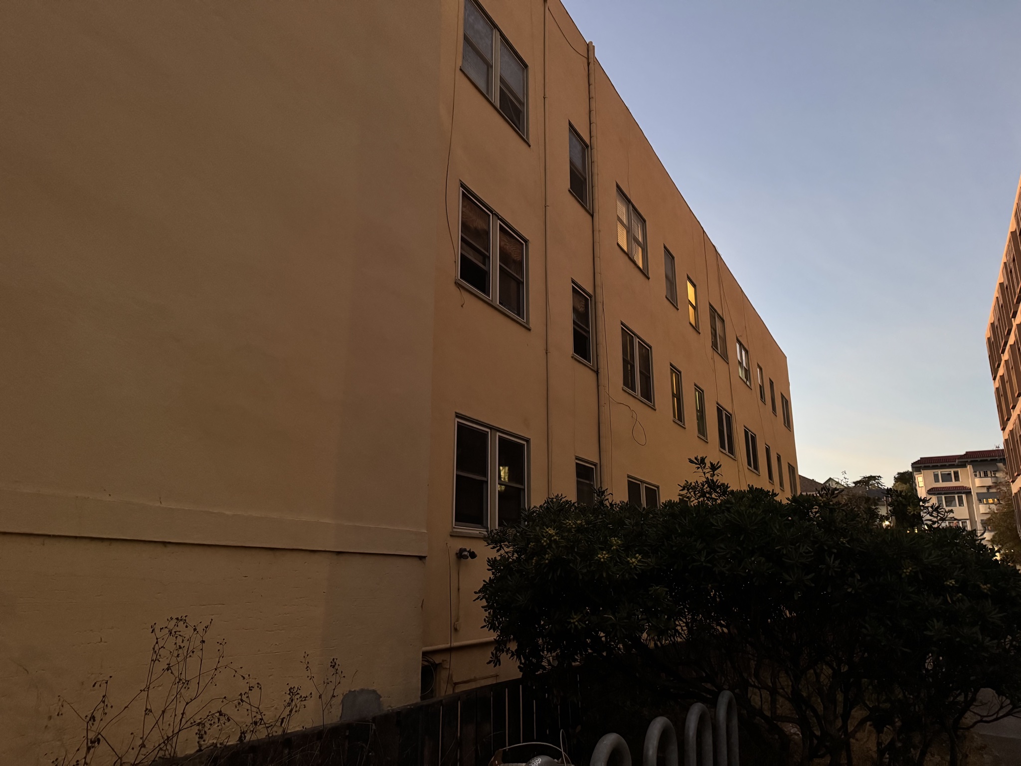
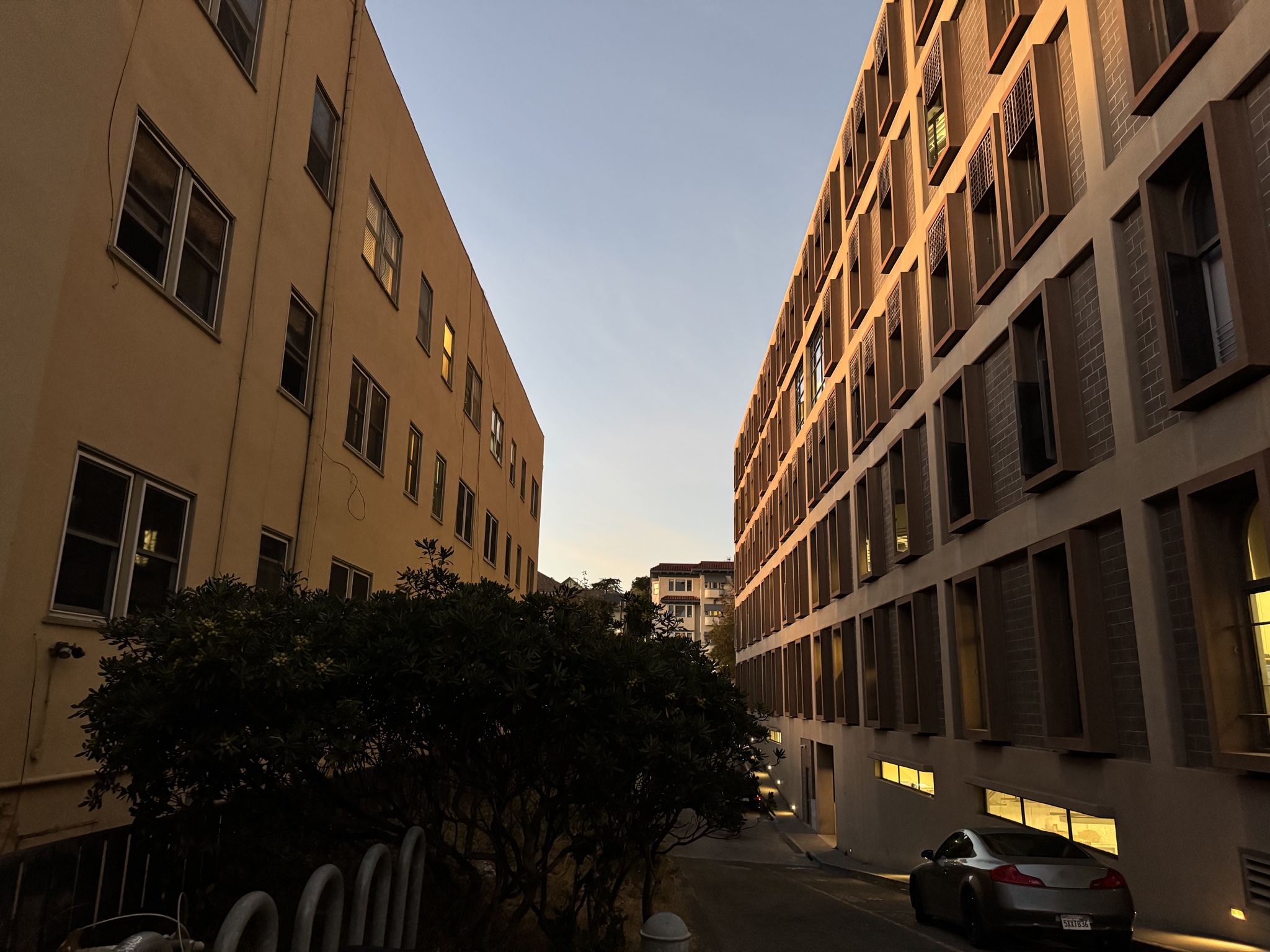
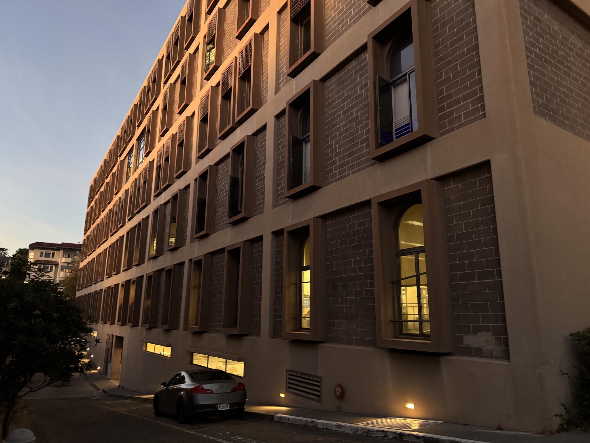
3b. Original Images

3b.i. The Wall

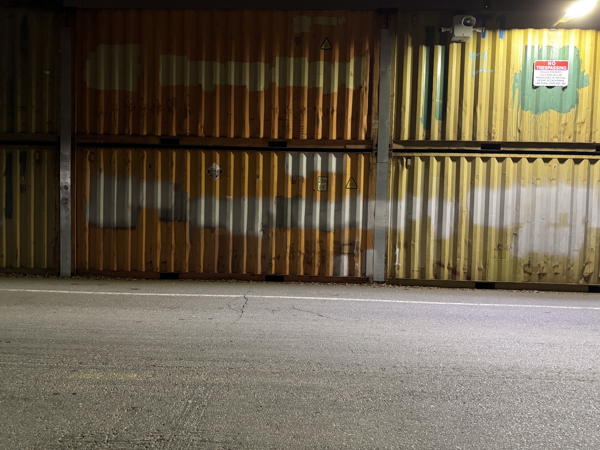
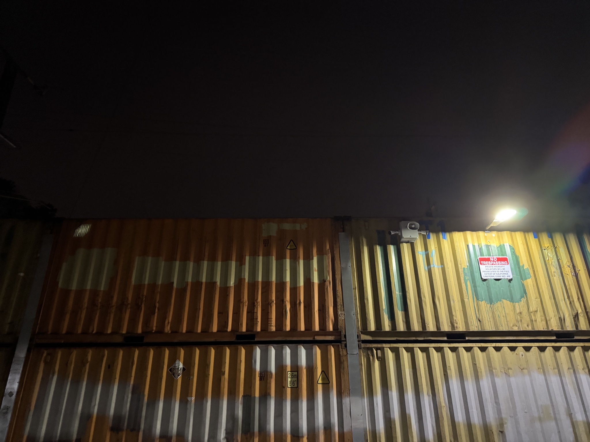
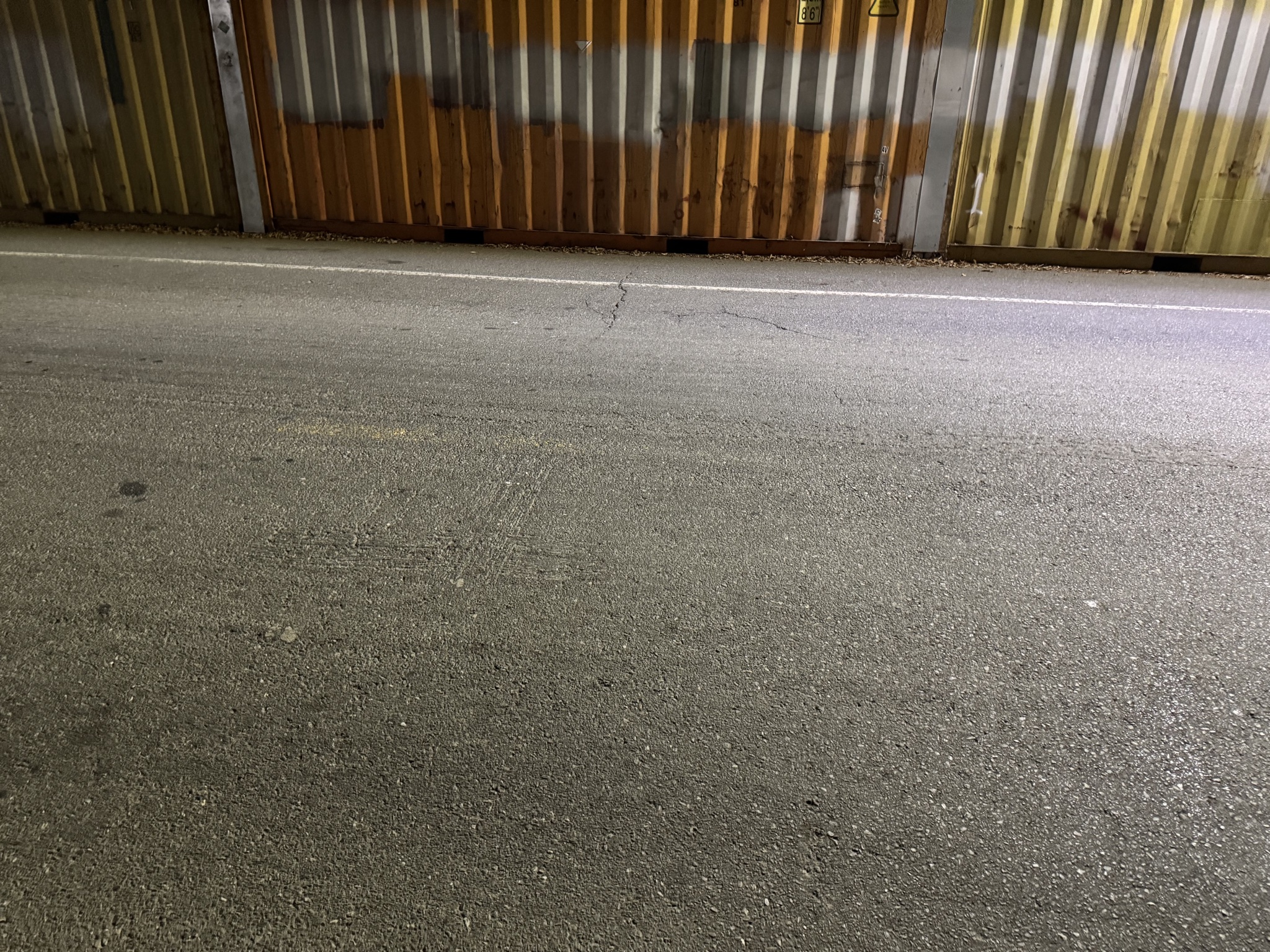
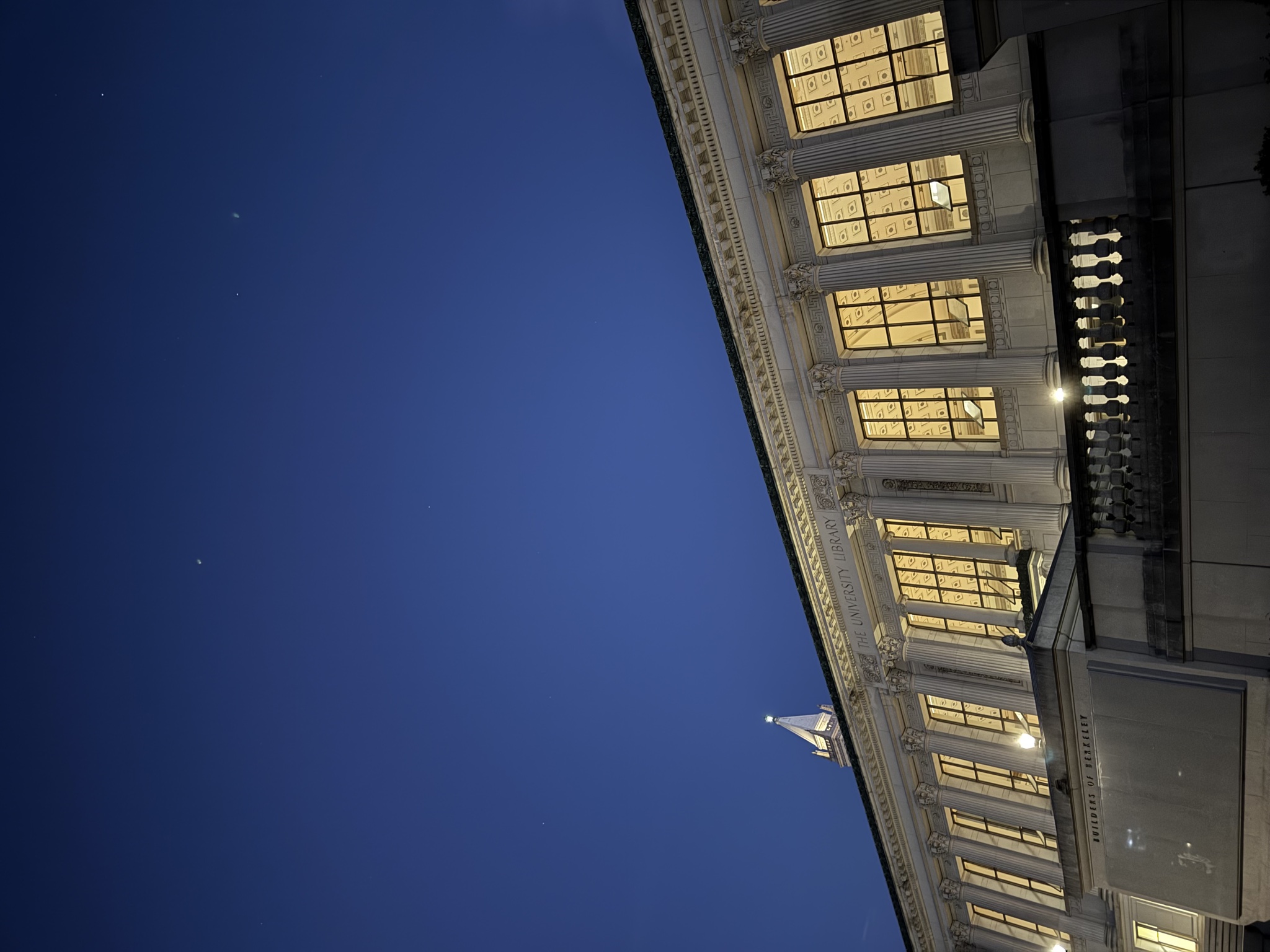
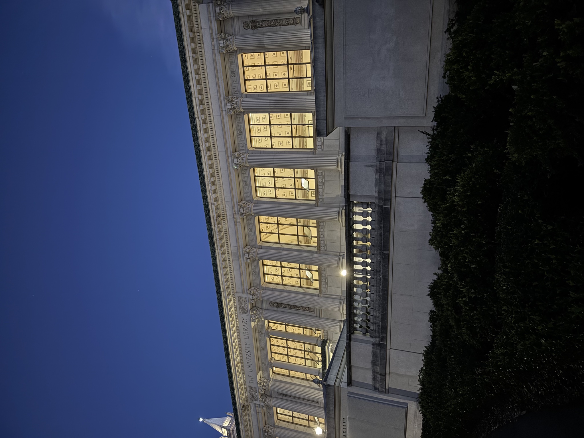
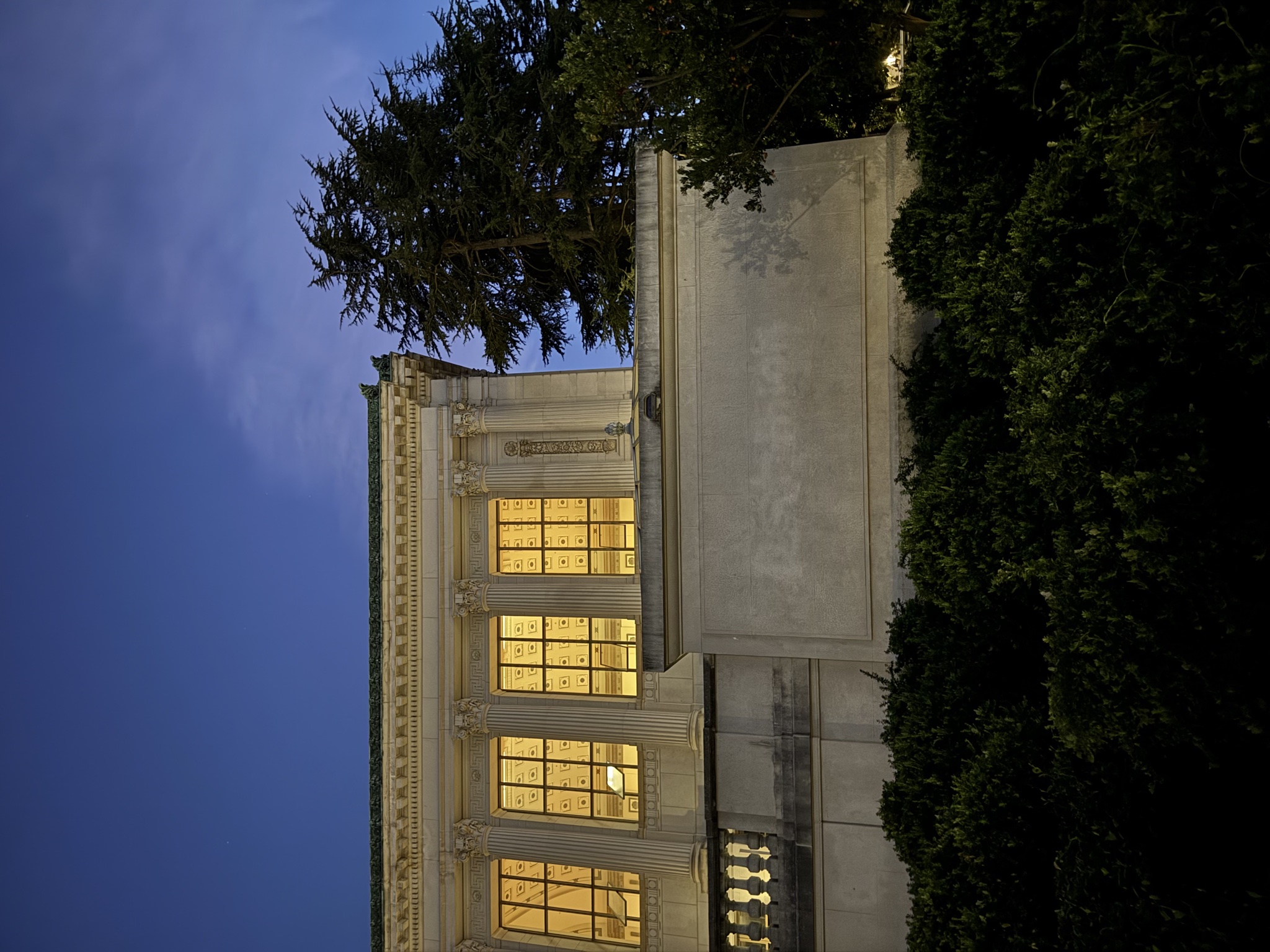
3b.ii. Doe at Night

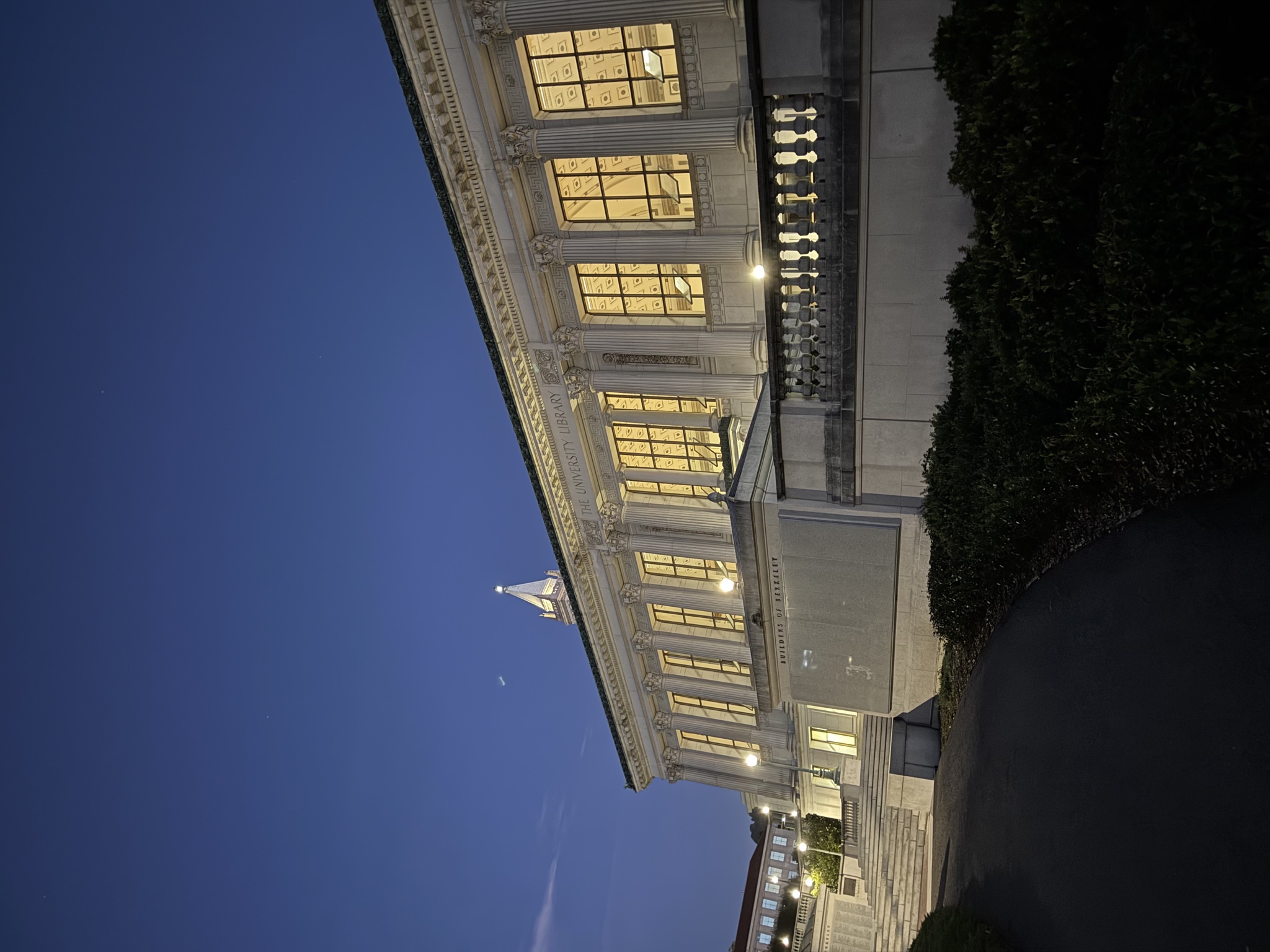
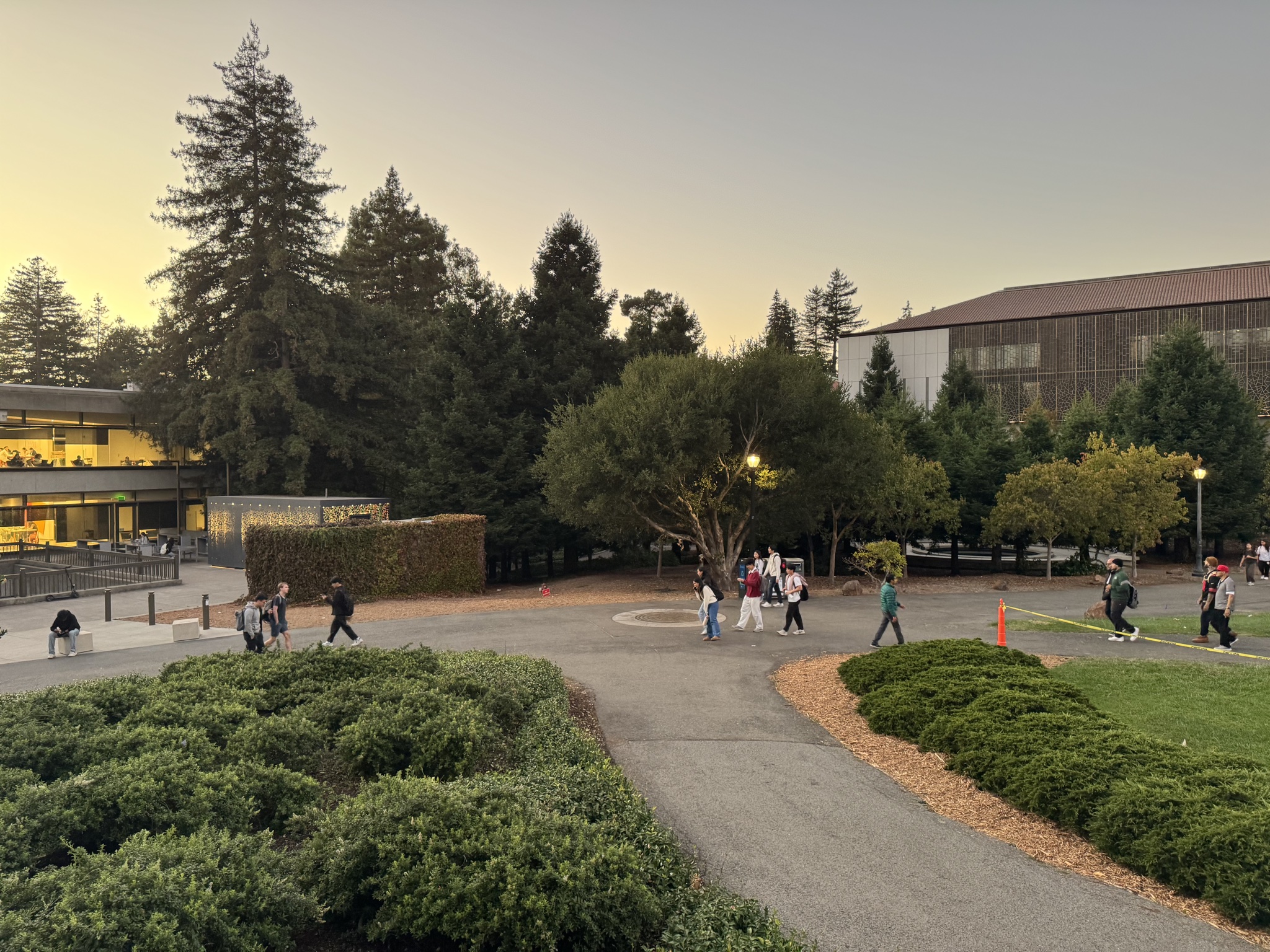
3b.iii. View from Doe

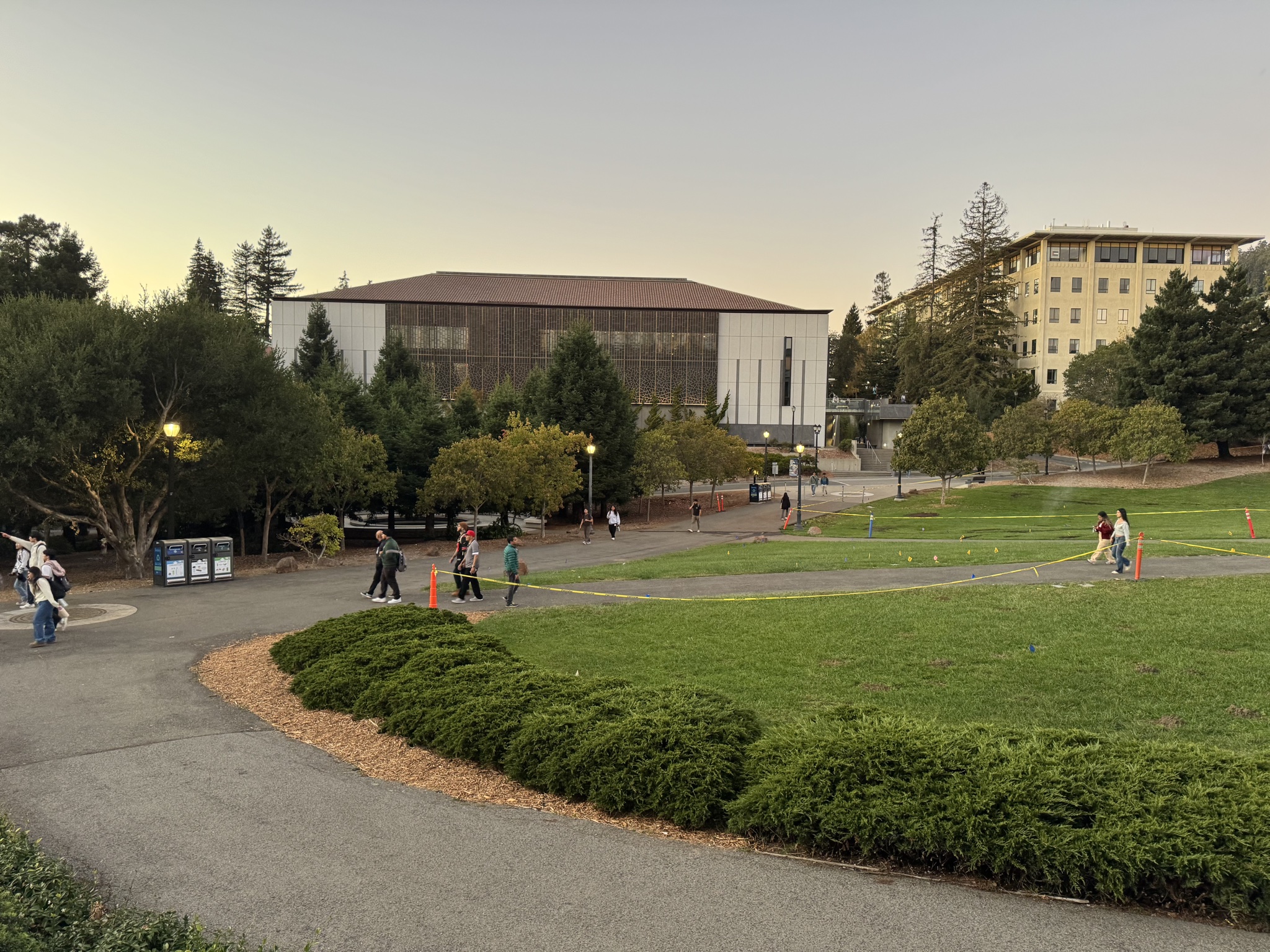
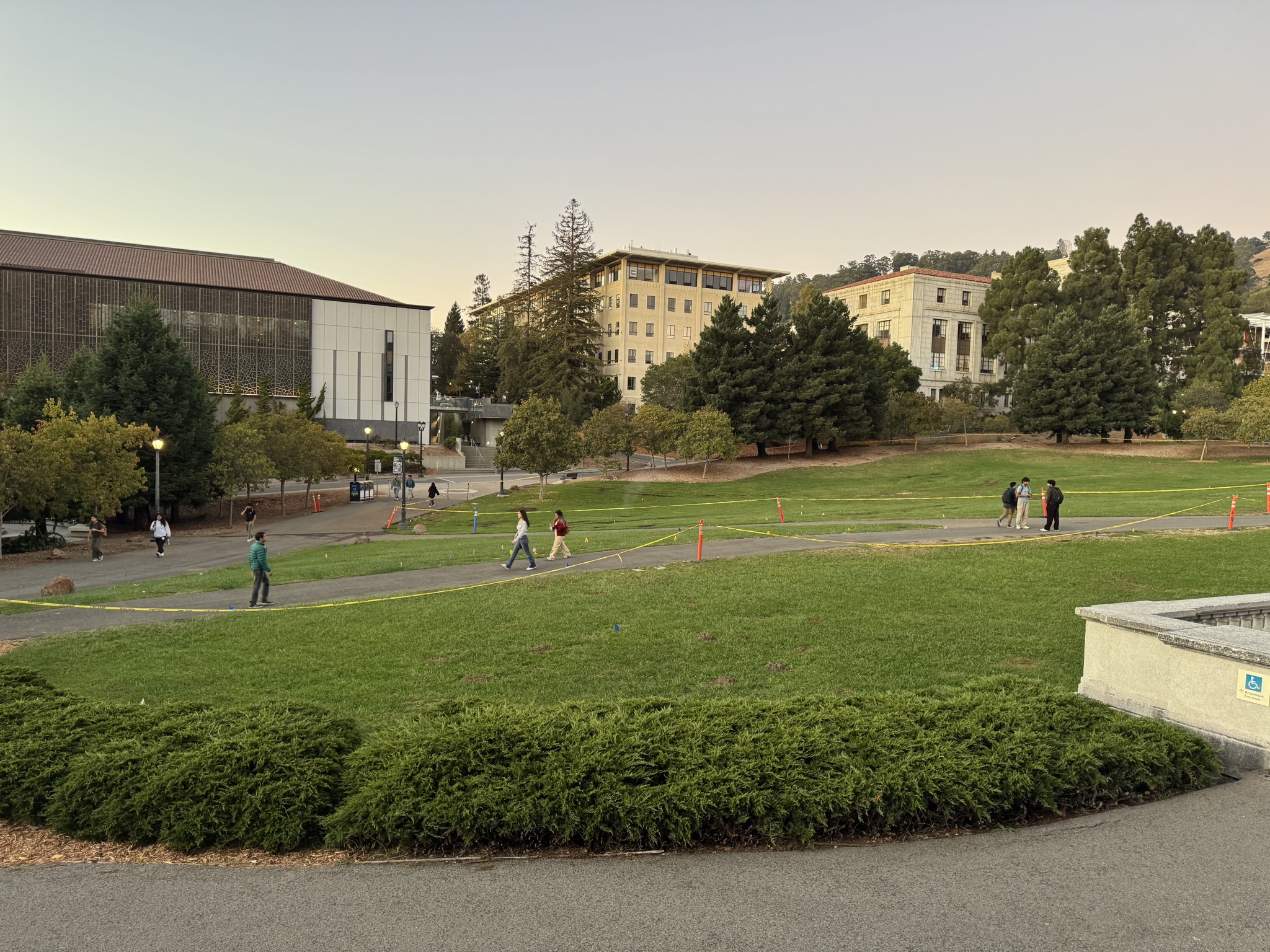
3b.iv. VLSB at Sunset

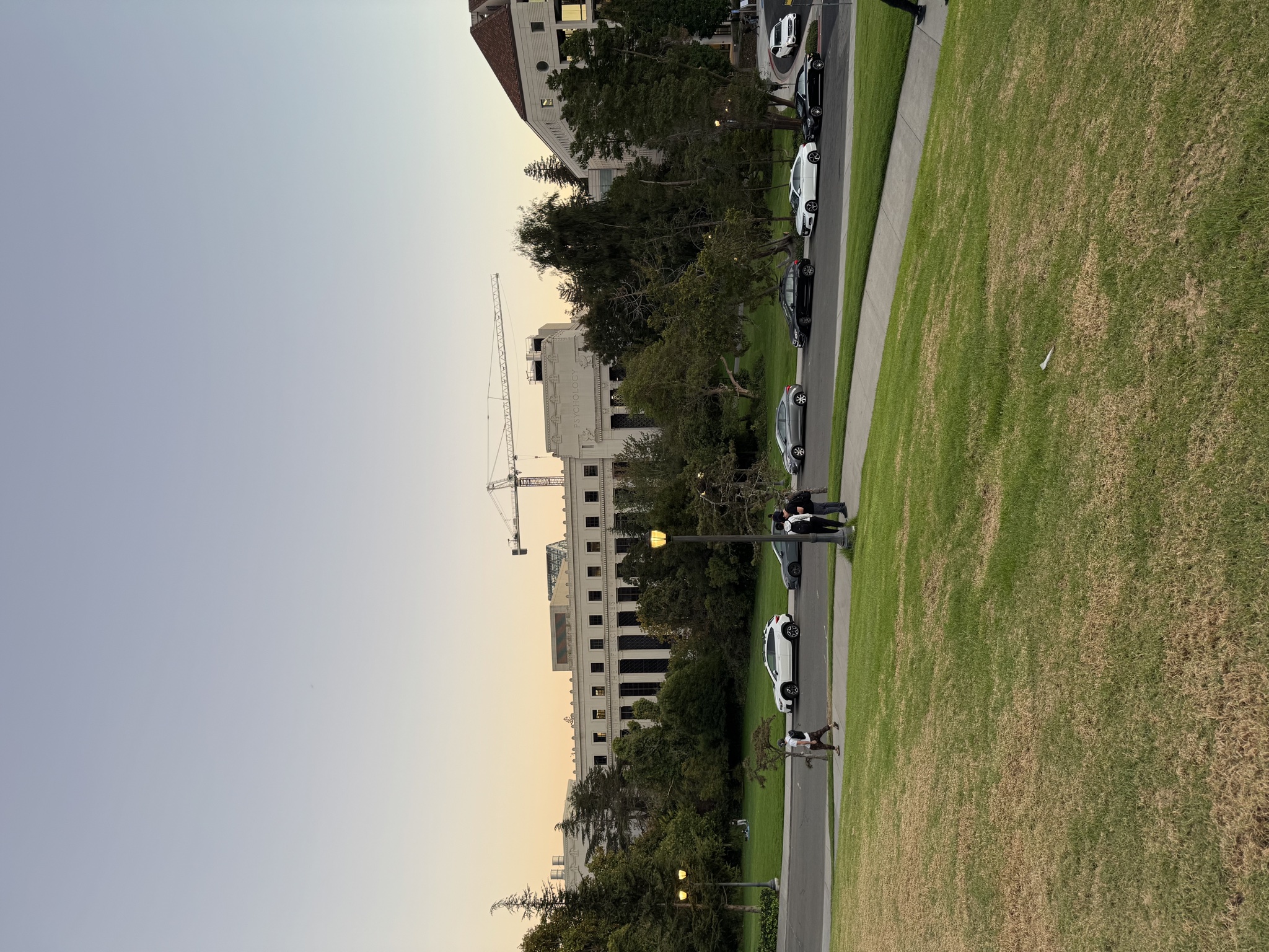
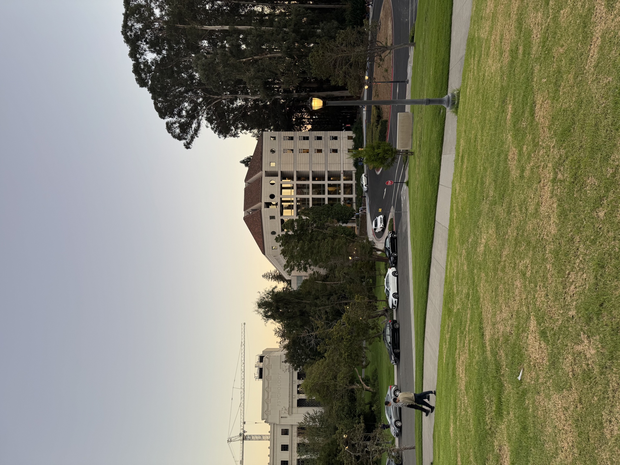
3b. v. Etcheverry Alley